# effect estimate and SE
hr_ext <- 0.65
se_ext <- sqrt(4 / 30)Update assurance of a clinical trial after not stopping at an interim analysis: time-to-event endpoint
Setup
We assume that DDCP at the design stage has already been computed, as described in the corresponding tutorial.
The question we are answering here is now how the two DDCP values (one for each prior), 0.70 and 0.59, change during the trial when one of the following events happens:
- External information on the treatment effect becomes available.
- An interim analysis for futility and/or efficacy for the trial of interest itself is performed, and the trial is not stopped at that interim analysis. The question then is how the knowledge of not stopping at the interim analysis changes the Bayesian predictive probability. Computations are possible for both scenarios, when the interim effect estimate is known or unknown to the sponsor.
External information becomes available
Assume an early phase trial on a related molecule has read out. How should we update DDCP? A Cox regression of this trial showed the following results:
As discussed in Section 2.4 of Rufibach et al. (2016) the proposal is to simply update our prior distribution \(q\) with this data. If we have more than one external trial result we can either do this updating sequentially or by first meta-analyzing the multiple trials.
# ----------------------------------
# Normal prior:
# ----------------------------------
up1 <- NormalNormalPosterior(datamean = log(hr_ext), sigma = se_ext, n = 1, nu = log(hr0),
                             tau = sd0)

bpp1 <- bpp_t2e(prior = "normal", successHR = hrMDD, d = nevents,
                priorHR = exp(up1$postmean), priorsigma = up1$postsigma)

# Normal prior
up1
$postmean
[1] -0.3844654
$postsigma
[1] 0.2236068bpp1[1] 0.7711889We find that updating the prior with the information from the external trial changes our Normal prior with exp(mean) = 0.70 and standard deviation 0.28 to a posterior with exp(mean) = hazard ratio of exp(-0.38) = 0.68 and increases DDCP from the initial 0.70 to 0.77.
# ----------------------------------
# pessimistic prior
# ----------------------------------
propA <- 0.5
fac <- (propA * (1 - propA)) ^ (-1)
finalSE <- sqrt(fac / nevents)
bpp1_1 <- integrate(FlatNormalPosterior, lower = -Inf, upper = Inf, successmean = log(hrMDD),
                    finalSE = finalSE, interimmean = log(hr_ext), interimSE = se_ext,
                    priormean = log(hr0flat), width = width1, height = height1)$value

# flat prior
bpp1_1
[1] 0.7089038We find that updating the prior with the information from the external trial increases DDCP from the initial 0.59 to 0.71 if we use the pessimistic prior.
Update the prior distribution after not stopping at an interim analysis
Now, the next milestone in our trial of interest is an interim analysis for both, futility and efficacy:
# ---------------------------------------------------
# specifications for the interim analysis
# ---------------------------------------------------

# local significance levels based on rpact output
alphas <- 2 * design$stageLevels
alphas
[1] 0.003050646 0.048999543# number of events
nevents <- ceiling(as.vector(sampleSize$eventsPerStage))
nevents[1] 191 381# MDDs at interim and final based on rpact output
hrMDD <- as.vector(sampleSize$criticalValuesEffectScaleLower)
hrMDD[1] 0.6508829 0.8172823# efficacy boundary --> MDD at interim analysis
effi <- hrMDD[1]
# futility boundary --> chosen informally
futi <- 1The interim analysis is planned after 191 events, using local significance levels of \(\alpha_{inte} \ = \ 0.003\) for the interim and \(\alpha_{fin} \ = \ 0.049\) for the final analysis. From these local significance levels, together with the number of events at each analysis, the minimal detectable differences (the hazard ratios corresponding to the critical values of the logrank test, MDD) can be derived. These are 0.651 and 0.817.
In addition to the interim efficacy analysis, assume that a futility analysis was pre-specified in the iDMC charter, with interim futility boundary of \(\theta_{fut} \ = \ \log(1)\). Thus, if the trial is not stopped at the interim analysis, we may assume for the log hazard ratio estimate at the interim analysis that \({\hat \theta}_{inte} \in [\theta_{eff}, \theta_{fut}] \ = \ [\log(0.651), \log(1)]\).
Now we are interested how DDCP changes if we do not stop at that interim analysis. For illustrative purposes, we assess various scenarios: interim is set up with futility and efficacy boundary, only one of the two, and we also provide updates using conditional power for the two extreme cases, namely that the estimate at the interim was known to be either equal to the futility or the efficacy boundary. Let us start with the Normal prior:
# ----------------------------------
# compute bpp after not stopping at interim, for Normal prior and various
# assumptions on the amount of information we learn at the interim
# ----------------------------------

# assuming we do not stop at a blinded interim analysis for futility and efficacy:
bpp3.tmp <- bpp_1interim_t2e(prior = "normal", successHR = hrMDD[2], d = nevents,
                          IntEffBoundary = effi, IntFutBoundary = futi, IntFixHR = 1,
                          priorHR = exp(up1$postmean), propA = 0.5, thetas = thetas,
                          priorsigma = up1$postsigma)

bpp3 <- bpp3.tmp$"BPP after not stopping at interim interval"
post3 <- bpp3.tmp$"posterior density interval"

# assuming we do not stop at a blinded interim analysis for efficacy only:
bpp3_effi_only <- bpp_1interim_t2e(prior = "normal", successHR = hrMDD[2], d = nevents,
                          IntEffBoundary = effi, IntFutBoundary = Inf, IntFixHR = 1,
                          priorHR = exp(up1$postmean), propA = 0.5, thetas = thetas,
                          priorsigma = up1$postsigma)$"BPP after not stopping at interim interval"

# assuming we do not stop at a blinded interim analysis for futility only:
bpp3_futi_only <- bpp_1interim_t2e(prior = "normal", successHR = hrMDD[2], d = nevents,
                          IntEffBoundary = 0, IntFutBoundary = futi, IntFixHR = 1,
                          priorHR = exp(up1$postmean), propA = 0.5, thetas = thetas,
                          priorsigma = up1$postsigma)$"BPP after not stopping at interim interval"

# assuming we do not stop at an unblinded interim where we observe exactly the efficacy boundary
# (IntFix = effi):
bpp4.tmp <- bpp_1interim_t2e(prior = "normal", successHR = hrMDD[2], d = nevents,
                          IntEffBoundary = 0, IntFutBoundary = Inf, IntFixHR = effi,
                          priorHR = exp(up1$postmean), propA = 0.5, thetas = thetas,
                          priorsigma = up1$postsigma)
bpp4 <- bpp4.tmp$"BPP after not stopping at interim exact"[2, 1]
post4 <- bpp4.tmp$"posterior density exact"[, 1]

# assuming we do not stop at an unblinded interim where we observe exactly the futility boundary
# (IntFix = futi):
bpp5.tmp <- bpp_1interim_t2e(prior = "normal", successHR = hrMDD[2], d = nevents,
                          IntEffBoundary = 0, IntFutBoundary = Inf, IntFixHR = futi,
                          priorHR = exp(up1$postmean), propA = 0.5, thetas = thetas,
                          priorsigma = up1$postsigma)
bpp5 <- bpp5.tmp$"BPP after not stopping at interim exact"[2, 1]
post5 <- bpp5.tmp$"posterior density exact"     # same as post4[, 2]
And the same for the pessimistic prior:
# ----------------------------------
# compute bpp after not stopping at interim, for pessimistic prior and various
# assumptions on the amount of information we learn at the interim
# here we do not assume an update with external studies, i.e. we use the
# initial prior
#
# Note that if we are only interested on a "blinded" or "interval" update we can set
# IntFix to an arbitrary value. Below, this is the case whenever we set IntFix = 1
# ----------------------------------

# assuming we do not stop at a blinded interim analysis for futility and efficacy:
bpp3.tmp_1 <- bpp_1interim_t2e(prior = "flat", successHR = hrMDD[2], d = nevents,
                               IntEffBoundary = effi, IntFutBoundary = futi, IntFixHR = 1,
                               priorHR = hr0, propA = 0.5, thetas = thetas,
                               width = width1, height = height1)

bpp3_1 <- bpp3.tmp_1$"BPP after not stopping at interim interval"
post3_1 <- bpp3.tmp_1$"posterior density interval"

# assuming we do not stop at a blinded interim analysis for efficacy only:
bpp3_1_effi_only <- bpp_1interim_t2e(prior = "flat", successHR = hrMDD[2], d = nevents,
                               IntEffBoundary = effi, IntFutBoundary = Inf, IntFixHR = 1,
                               priorHR = hr0, propA = 0.5, thetas = thetas, width = width1,
                               height = height1)$"BPP after not stopping at interim interval"

# assuming we do not stop at a blinded interim analysis for futility only:
bpp3_1_futi_only <- bpp_1interim_t2e(prior = "flat", successHR = hrMDD[2], d = nevents,
                               IntEffBoundary = 0, IntFutBoundary = futi, IntFixHR = 1,
                               priorHR = hr0, propA = 0.5, thetas = thetas, width = width1,
                               height = height1)$"BPP after not stopping at interim interval"

# assuming we do not stop at an unblinded interim where we observe exactly the efficacy boundary
# (IntFix = effi):
bpp4_1.tmp <- bpp_1interim_t2e(prior = "flat", successHR = hrMDD[2], d = nevents,
                               IntEffBoundary = 0, IntFutBoundary = Inf, IntFixHR = effi,
                               priorHR = hr0, propA = 0.5, thetas = thetas, width = width1,
                               height = height1)
bpp4_1 <- bpp4_1.tmp$"BPP after not stopping at interim exact"[2, 1]
post4_1 <- bpp4_1.tmp$"posterior density exact"

# assuming we do not stop at an unblinded interim where we observe exactly the futility boundary
# (IntFix = futi):
bpp5_1 <- integrate(Vectorize(estimate_toIntegrate), lower = -Inf, upper = Inf, prior = "flat",
                    successmean = log(hrMDD[2]), finalSE = finalSE, interimmean = log(futi),
                    interimSE = sqrt(fac / nevents[1]), priormean = log(hr0),
                    width = width1, height = height1)$value

bpp5_1.tmp <- bpp_1interim_t2e(prior = "flat", successHR = hrMDD[2], d = nevents,
                               IntEffBoundary = 0, IntFutBoundary = Inf, IntFixHR = futi,
                               priorHR = hr0, propA = 0.5, thetas = thetas, width = width1,
                               height = height1)
bpp5_1 <- bpp5_1.tmp$"BPP after not stopping at interim exact"[2, 1]
post5_1 <- bpp5_1.tmp$"posterior density exact"
Posterior densities
The resulting posteriors after the update with the external trial is depicted below. We also add to the figures the posterior after not stopping at the interim analysis that considers the efficacy and futility boundary, i.e. we may assume that \[{\hat \theta}_{inte} \in [\theta_{eff}, \theta_{fut}] \ = \ [\log(0.651), \log(1)].\]
These figures adapt Figure 1 in Rufibach et al. (2016) to our numbers.
par(las = 1, mar = c(9, 5, 2, 1), mfrow = c(1, 2), cex = 0.8)
leg <- c("prior", "posterior after external trial",
         "posterior after external trial and\nnot stopping at interim")

# ----------------------------------
# Normal prior:
# ----------------------------------
plot(0, 0, type = "n", xlim = xli, ylim = yli, xlab = "", ylab = "density",
     main = "")
title(expression("Normal prior density and posteriors for "*theta), line = 0.7)
basicPlot(leg = FALSE, IntEffBoundary = log(effi), IntFutBoundary = log(futi),
          successmean = log(hrMDD), priormean = log(hr0))
lines(lthetas, dnorm(lthetas, mean = log(hr0), sd = sd0), col = 2, lwd = 2)
lines(lthetas, dnorm(lthetas, mean = up1$postmean, sd = up1$postsigma), col = 3, lwd = 2)
lines(lthetas, post3, col = 1, lwd = 2)
legend(-1.2, yli[2], leg, lty = 1, col = c(2:3, 1), bty = "n", lwd = 2)

# ----------------------------------
# pessimistic prior:
# ----------------------------------

# first we have to compute the posteriors after the external updates:
flatpost1 <- rep(NA, length(thetas))
for (i in 1:length(thetas)){
  flatpost1[i] <- estimate_posterior(x = lthetas[i], prior = "flat", interimmean = log(hr_ext),
                                     interimSE = se_ext, priormean = log(hr0flat), width = width1,
                                     height = height1)
}

plot(0, 0, type = "n", xlim = xli, ylim = yli, xlab = "", ylab = "density", main = "")
title(expression("Flat prior density and posteriors for "*theta), line = 0.7)
basicPlot(leg = FALSE, IntEffBoundary = log(effi), IntFutBoundary = log(futi),
          successmean = log(hrMDD), priormean = log(hr0flat))
lines(lthetas, dUniformNormalTails(lthetas, mu = log(hr0flat), width = width1, height = height1),
      lwd = 2, col = 2)
lines(lthetas, flatpost1, col = 3, lwd = 2)
lines(lthetas, post3_1, col = 1, lwd = 2)

legend(-1.2, yli[2], leg, lty = 1, col = c(2:3, 1), bty = "n", lwd = 2)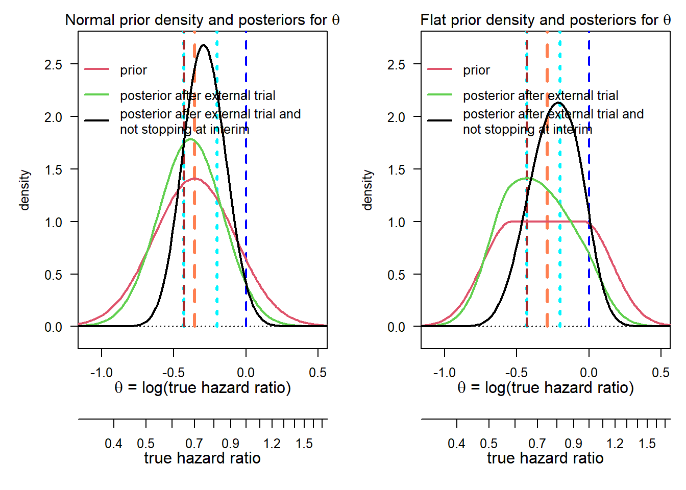
Next, we also provide the posteriors after updating with the interim information assuming the effect estimate at the interim came to lie on one of the interim boundaries:
par(las = 1, mar = c(9, 5, 4, 1), mfrow = c(1, 2), cex = 0.8)

# ----------------------------------
# Normal prior:
# ----------------------------------
plot(0, 0, type = "n", xlim = xli, ylim = c(yli[1], 3.5), xlab = "", ylab = "density",
     main = "")
title("Posteriors for after not stopping\nat interim, Normal prior", line = 0.7)
basicPlot(leg = FALSE, IntEffBoundary = log(effi), IntFutBoundary = log(futi),
          successmean = log(hrMDD), priormean = log(hr0))
lines(lthetas, post3, col = 1, lwd = 2)
lines(lthetas, post4, col = 2, lwd = 2)
lines(lthetas, post5, col = 3, lwd = 2)
leg2 <- c("interval knowledge", expression(hat(theta)*" = efficacy boundary"),
          expression(hat(theta)*" = futility boundary"))
legend(-1, 3.5, leg2, lty = 1, col = 1:3, lwd = 2, bty = "n",
       title = "posterior after not stopping at interim,")

# ----------------------------------
# pessimistic prior:
# ----------------------------------
plot(0, 0, type = "n", xlim = xli, ylim = c(yli[1], 3.5), xlab = "", ylab = "density",
     main = "")
title("Posteriors after not stopping\nat interim, pessimistic prior", line = 0.7)
basicPlot(leg = FALSE, IntEffBoundary = log(effi), IntFutBoundary = log(futi),
          successmean = log(hrMDD[2]), priormean = log(hr0flat))
lines(lthetas, post3_1, col = 1, lwd = 2)
lines(lthetas, post4_1, col = 2, lwd = 2)
lines(lthetas, post5_1, col = 3, lwd = 2)
legend(-1, 3.5, leg2, lty = 1, col = 1:3, lwd = 2, bty = "n",
       title = "posterior after not stopping at interim,")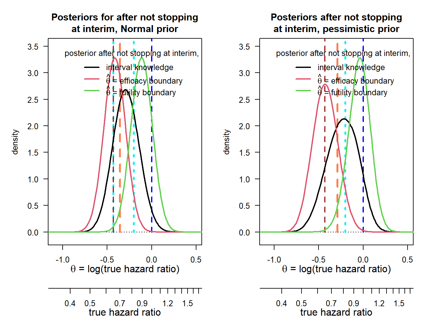
Table 1 in Rufibach et al. (2016)
Finally, we collect all the results computed above in one table, adapting Table 1 in Rufibach et al. (2016).
mat <- matrix(NA, ncol = 2, nrow = 9)
mat[, 1] <- c(pnorm1, pnorm2, bpp0, bpp1, bpp3, bpp3_futi_only, bpp3_effi_only, bpp4, bpp5)
mat[, 2] <- c(flat1, flat2, bpp0_1, bpp1_1, bpp3_1, bpp3_1_futi_only, bpp3_1_effi_only,
              bpp4_1, bpp5_1)
colnames(mat) <- c("Normal prior", "Flat prior")
rownames(mat) <- c(paste("Probability for hazard ratio to be $\\le$ ", lims[1], sep = ""),
paste("Probability for hazard ratio to be $\\ge$ ", lims[2], sep = ""),
"DDCP based on prior distribution", "DDCP after external trial",
"DDCP after external trial and not stopping at interim, assuming $\\hat \\theta \\in [\\theta_{eff}, \\theta_{fut}]$",
"DDCP after external trial and not stopping at interim, assuming $\\hat \\theta \\in [-\\infty, \\theta_{fut}]$",
"DDCP after external trial and not stopping at interim, assuming $\\hat \\theta \\in [\\theta_{eff}, \\infty]$",
"DDCP after external trial and not stopping at interim, assuming $\\hat \\theta = \\theta_{eff}$",
"DDCP after external trial and not stopping at interim, assuming $\\hat \\theta = \\theta_{fut}$")
mat <- as.data.frame(format(mat, digits = 2))
knitr::kable(mat)| Normal prior | Flat prior | |
|---|---|---|
| Probability for hazard ratio to be \(\le\) 0.5 | 0.117 | 0.109 |
| Probability for hazard ratio to be \(\ge\) 1 | 0.104 | 0.213 |
| DDCP based on prior distribution | 0.697 | 0.586 |
| DDCP after external trial | 0.771 | 0.709 |
| DDCP after external trial and not stopping at interim, assuming \(\hat \theta \in [\theta_{eff}, \theta_{fut}]\) | 0.685 | 0.560 |
| DDCP after external trial and not stopping at interim, assuming \(\hat \theta \in [-\infty, \theta_{fut}]\) | 0.832 | 0.786 |
| DDCP after external trial and not stopping at interim, assuming \(\hat \theta \in [\theta_{eff}, \infty]\) | 0.597 | 0.397 |
| DDCP after external trial and not stopping at interim, assuming \(\hat \theta = \theta_{eff}\) | 0.990 | 0.987 |
| DDCP after external trial and not stopping at interim, assuming \(\hat \theta = \theta_{fut}\) | 0.062 | 0.031 |
Update of DDCP when not stopping the trial in two blinded interim analyses
The theory developed in Rufibach et al. (2016) can straightforwardly be extended to accomodate more than one interim analysis. Below, we illustrate the DDCP update assuming a trial that did not stop after first a futility and second an efficacy interim analysis. Note that the function bpp_2interim in the package bpp Rufibach, Jordan, and Abt (2021) so far only allows specification of a Normal prior and does not have the option to specify exact knowledge of the interim boundary (argument IntFix in bpp_1interim). If you want to approximate the case that you actually know the interim estimate then you can chose identical upper and lower interval limits for the arguments IntEffBoundary and IntFutBoundary.
We use the Gallium trial Marcus et al. (2017) for illustration, see also this rpact tutorial.
Note that bpp does not offer a wrapper (yet) for this scenario, that is why we need to embed the question in the generic syntac of bpp_2interim and define some additional quantities.
# ------------------------------------------------------------------------------------------
# Illustrate the update after two passed interims using the Gallium clinical trial
# ------------------------------------------------------------------------------------------

# mean and sd of Normal prior:
hr0 <- 0.9288563
priormean <- log(hr0)
priorsigma <- sqrt(4 / 12)

# specifications for pivotal study:
propA <- 0.5
fac <- (propA * (1 - propA)) ^ (-1)

nevents <- c(113, 245, 370)
dataSE <- sqrt(fac / nevents[1:2])
finalSE <- sqrt(fac / nevents[3])

design_ga <- getDesignGroupSequential(informationRates = nevents / max(nevents),
    typeOfDesign = "asOF", sided = 1, alpha = 0.025,
    futilityBounds = c(0, -6), bindingFutility = FALSE)
sampleSize_ga <- getSampleSizeSurvival(design = design_ga, hazardRatio = 6 / 8.1)
hrMDD <- sampleSize_ga$criticalValuesEffectScale[, 1]
successmean <- log(hrMDD[3])

# 2-d vector of efficacy and futility interim boundaries:
effi <- log(c(0, hrMDD[2]))  # 1st interim is for futility only, no stopping for efficacy possible
futi <- log(c(1, Inf))       # 2nd interim is for efficacy only, no stopping for futility possible

bpp2 <- bpp_2interim(prior = "normal", interimSE = dataSE, finalSE = finalSE,
             successmean = successmean, IntEffBoundary = effi, IntFutBoundary = futi,
             priormean = log(hr0), thetas = lthetas, priorsigma = priorsigma)

bpp2$"initial BPP"
[1] 0.4107881bpp2$"BPP after not stopping at interim interval"[1] 0.3311625So the DDCP decreases from its initial value of 0.41 to 0.33 after neither stopping at the futility nor the efficacy interim.
References
Marcus, R., A. Davies, K. Ando, W. Klapper, S. Opat, C. Owen, E. Phillips, et al. 2017. “Obinutuzumab for the First-Line Treatment of Follicular Lymphoma.” N. Engl. J. Med. 377 (14): 1331–44.
Rufibach, K., P. Jordan, and M. Abt. 2016. “Sequentially updating the likelihood of success of a Phase 3 pivotal time-to-event trial based on interim analyses or external information.” J Biopharm Stat 26 (2): 191–201. http://dx.doi.org/10.1080/10543406.2014.972508.
———. 2021. Bpp: Computations Around Bayesian Predictive Power.