# Load necessary packages
library(phase1b)Applying the UNICYCLE framework: RO7172508 and ADAs
Setup
The study
This page provides the details of a Bayesian posterior probability computation to enable decision-making for the impact of anti-drug-antibodies (ADAs) on exposure of RO7172508 during a dose escalation study followed by expansion cohorts. Throughout the study, the incidence and titer of ADAs as well as the pharmacokinetic of RO7172508 will be assessed on an ongoing basis. If a relevant number of participants experience a relevant loss of exposure, then obinutuzumab pre-treatment will be implemented. Notice that it is assumed that, from the first cohort evaluated for ADAs, the dose level reached does not change the underline probability of developing ADAs.
The endpoint of interest is “relevant loss of exposure to RO7172508 due to ADAs” (denoted by “LOE+ rate”) and thus binary - the UNICYCLE framework is therefore applicable to this question.
Define the prior
We assume a \(\beta(a, b)\)-prior for the underlying LOE+ rate. The prior parameters are based on results observed in patients treated with RO6958688 (CEA-TCB) and were appropriately down weighted in order to derive the prior:
# total patients in CEA TCB trial
ceatot <- 21

# number of patients with loss of exposure in CEA TCB trial
cealoe <- 14

# define the prior parameters
a_prior <- round(cealoe / ceatot, 3)
b_prior <- round(1 - a_prior, 3)
c(a_prior, b_prior)
[1] 0.667 0.333This \(\beta(0.667, 0.333)\) density is depicted below:
par(las = 1, mar = c(4.5, 4, 3, 1))
x <- seq(0, 1, by = 0.0001)
bdens <- dbeta(x, a_prior, b_prior)
plot(x, bdens, type = "l", lwd = 2, col = "red", xlab = "LOE+ Rate",
     ylab = "Density", ylim = c(0,10), main = "prior")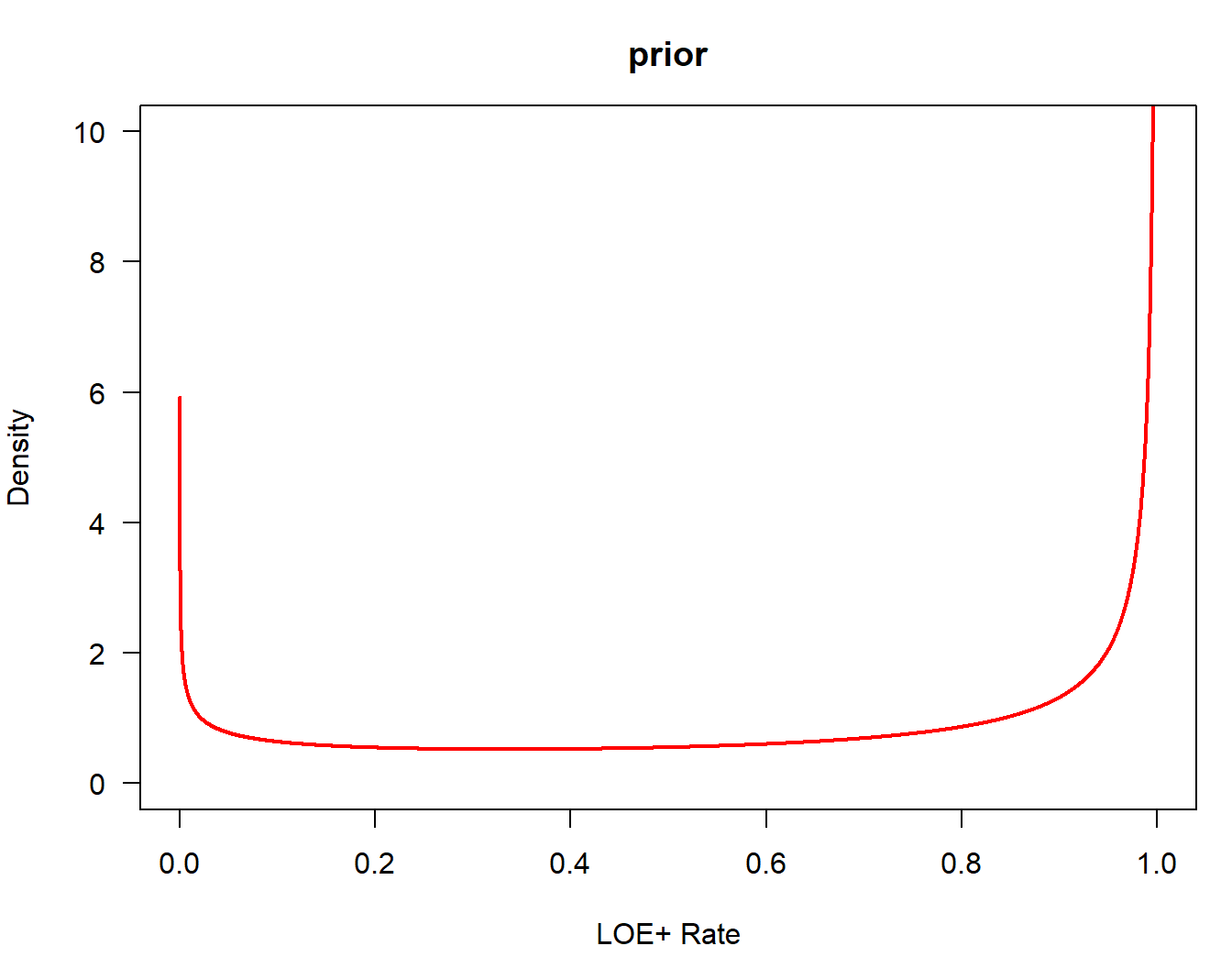
Posterior probabilities and decision criteria
As new information is collected the prior distribution will be updated to generate the posterior probability distribution of the true LOE+ rate, given the data observed. At each assessment the posterior probability, with \(n\) participants who experienced a relevant loss of exposure out of \(n + m\) additionally evaluable patients, will therefore (due to conjugancy of the beta-binomial model) again follow a beta distribution with parameters \(a + n\) and \(b + m\).
At the time of the evaluation, if there is high confidence that the underlying true LOE+ rate is above a pre-defined target then obinutuzumab pre-treatment will be introduced for all subsequent participants in the study. If the criteria is not met the dose escalation will proceed without obinutuzumab pre-treatment until the next assessment or the end of the dose escalation. To be more specific, for a given target LOE+ rate the posterior probability can be computed, following the notation of the UNICYCLE framework, as follows:
\[\begin{align*} PP &= \mathbb{P}(p_E>p_1) \\ &= \mathbb{P} (\text{True LOE+ Rate} \ge \text{Target LOE+ Rate} | \text{data, prior}). \end{align*}\]
So the decision rule is to implement obinutuzumab if \(PP ≥ t_U\) for some probability threshold \(t_U\), otherwise to continue.
# target rates
theta_h <- 0.8
theta_l <- 0.7

# probability thresholds
target_h <- 0.5
target_l <- 0.05
The target LOE+ rate has been set to 0.5 and the posterior probability threshold to \(t_U = 0.8\), based on what was considered an acceptable probability of implementing obinutuzumab under different assumptions on the true underling LOE+ rate, see the evaluation of operating characteristics below.
At the end of the dose escalation, if the above criteria have not yet been met and, at the same time, there is low confidence (meaning \(PP < 0.7\)) that the true underlying LOE+ rate is less than 0.05, then expansion cohorts with and without obinutuzumab will be evaluated. The expansion cohorts will determine if the safety profile and pharmacodynamics effects of the regimens are acceptable with continued RO7172508 exposure.
Evaluation of operating characteristics of the decision rule
# n patients for first evaluation
n1i <- 14
First evaluation with 14 patients
First, we compute the posterior probabilities for any given number of patients experiencing a loss of exposure:
postprob_n1i <-  postprob(x = c(0:n1i), n = n1i, p = target_h, parE = c(a_prior, b_prior))
tablepost<- as.data.frame(cbind(round(c(0:n1i), 0), round(postprob_n1i, 3)))
colnames(tablepost) <- c("n with LOE", "posterior probability")
knitr::kable(tablepost)| n with LOE | posterior probability |
|---|---|
| 0 | 0.000 |
| 1 | 0.000 |
| 2 | 0.004 |
| 3 | 0.018 |
| 4 | 0.064 |
| 5 | 0.164 |
| 6 | 0.329 |
| 7 | 0.535 |
| 8 | 0.733 |
| 9 | 0.877 |
| 10 | 0.957 |
| 11 | 0.989 |
| 12 | 0.998 |
| 13 | 1.000 |
| 14 | 1.000 |
So as an illustration, at the first evaluation after 14 patients we need to observe 9 or more participants with relevant loss of exposure to have a posterior probability equal or higher than 0.8 (\(\theta_U = 0.8\)) that the true LOE+ rate is \(\ge 0.5\).
Now, to evaluate the properties of this decision rule we define a function that simulates corresponding trials and computes the operating characteristics, based on the function ocPostprob in the phase1b package:
# define function that simulates posterior probabilities
myocpost <-  function(p0, p1, a_prior, b_prior, myN, mytU, mytL, nsim = 10 ^ 4){
  pgrid <- seq(from = 0, to = 1, by = 0.05)
  Probs <- expand.grid("nn" = myN, "tU" = mytU, "tL" = mytL, "p" = pgrid)
  resProbs <- data.frame(matrix(NA, ncol = 3, nrow = nrow(Probs)) )
  colnames(resProbs) <- c("goProbs", "stopProbs", "greyProbs")

  for (parRun in seq_len(nrow(Probs))){
    auxpar <- Probs[parRun, ]
    thisOc <- ocPostprob(nn = auxpar$nn,
                         p = auxpar$p,
                         p0 = p0,
                         p1 = p1,
                         tL = auxpar$tL,
                         tU = auxpar$tU,
                         parE = c(a_prior, b_prior),
                         ns = nsim,
                         nr = FALSE,
                         d = NULL)$oc

    resProbs[parRun, ] <- thisOc[ , c("PrEfficacy", "PrFutility", "PrGrayZone")]
  }

  TotProbs <- cbind(Probs, resProbs)
  return (TotProbs)
}
After having defined the function that simulates posterior probabilities let us apply it to our scenario.
# n patients for first evaluation
n1i <- 14

# number of simulation runs
nsim <- 10 ^ 4
Based on 14 initial patients and 10000 simulation runs, the posterior probability of taking the decision to implement obinutuzumab for a given true underlying LOE+ rate is illustrated in the table below.
set.seed(1234)
TotProbsA <- myocpost(p0 = 0, p1 = target_h, a_prior = a_prior, b_prior = b_prior,
                      myN = n1i, mytU = theta_h, mytL = 1, nsim = nsim)
TotProbsA
nn tU tL p goProbs stopProbs greyProbs
1 14 0.8 1 0.00 0.0000 0 1.0000
2 14 0.8 1 0.05 0.0000 0 1.0000
3 14 0.8 1 0.10 0.0000 0 1.0000
4 14 0.8 1 0.15 0.0000 0 1.0000
5 14 0.8 1 0.20 0.0003 0 0.9997
6 14 0.8 1 0.25 0.0010 0 0.9990
7 14 0.8 1 0.30 0.0082 0 0.9918
8 14 0.8 1 0.35 0.0249 0 0.9751
9 14 0.8 1 0.40 0.0584 0 0.9416
10 14 0.8 1 0.45 0.1239 0 0.8761
11 14 0.8 1 0.50 0.2159 0 0.7841
12 14 0.8 1 0.55 0.3327 0 0.6673
13 14 0.8 1 0.60 0.4906 0 0.5094
14 14 0.8 1 0.65 0.6381 0 0.3619
15 14 0.8 1 0.70 0.7830 0 0.2170
16 14 0.8 1 0.75 0.8890 0 0.1110
17 14 0.8 1 0.80 0.9585 0 0.0415
18 14 0.8 1 0.85 0.9904 0 0.0096
19 14 0.8 1 0.90 0.9985 0 0.0015
20 14 0.8 1 0.95 1.0000 0 0.0000
21 14 0.8 1 1.00 1.0000 0 0.0000Now plot these operating characteristics against the true assumed LOE+ rate:
matplot(TotProbsA$p, TotProbsA[, c("goProbs", "greyProbs")],
        xlab = '', xaxt = "n", ylab = 'Probability', type="l",
        col = c("red", "blue"), lty = c(1, 2), lwd = 3)
at <- seq(from = 0, to = 1, by = 0.1)
axis(side = 1, at = at)
abline(v = c(illu1, illu2), lty = 6, col = "orange")
legend ("left", c("Implement +Obinutuzumab", "Continue to Evaluate"),
        col = c("red", "blue"), lty = c(1, 2), bty = "n", lwd = 3)

title(sub = substitute(paste("Prior (", a, "," , b, "); ", "Target LOE+ rate high = ", h, "; ",
                              Theta[U], "= " , theta_h),
                       list(a = a_prior, b = b_prior, h = target_h, theta_h = theta_h)))
mtext(side = 1, 'True LOE+ Rate', line = 2) 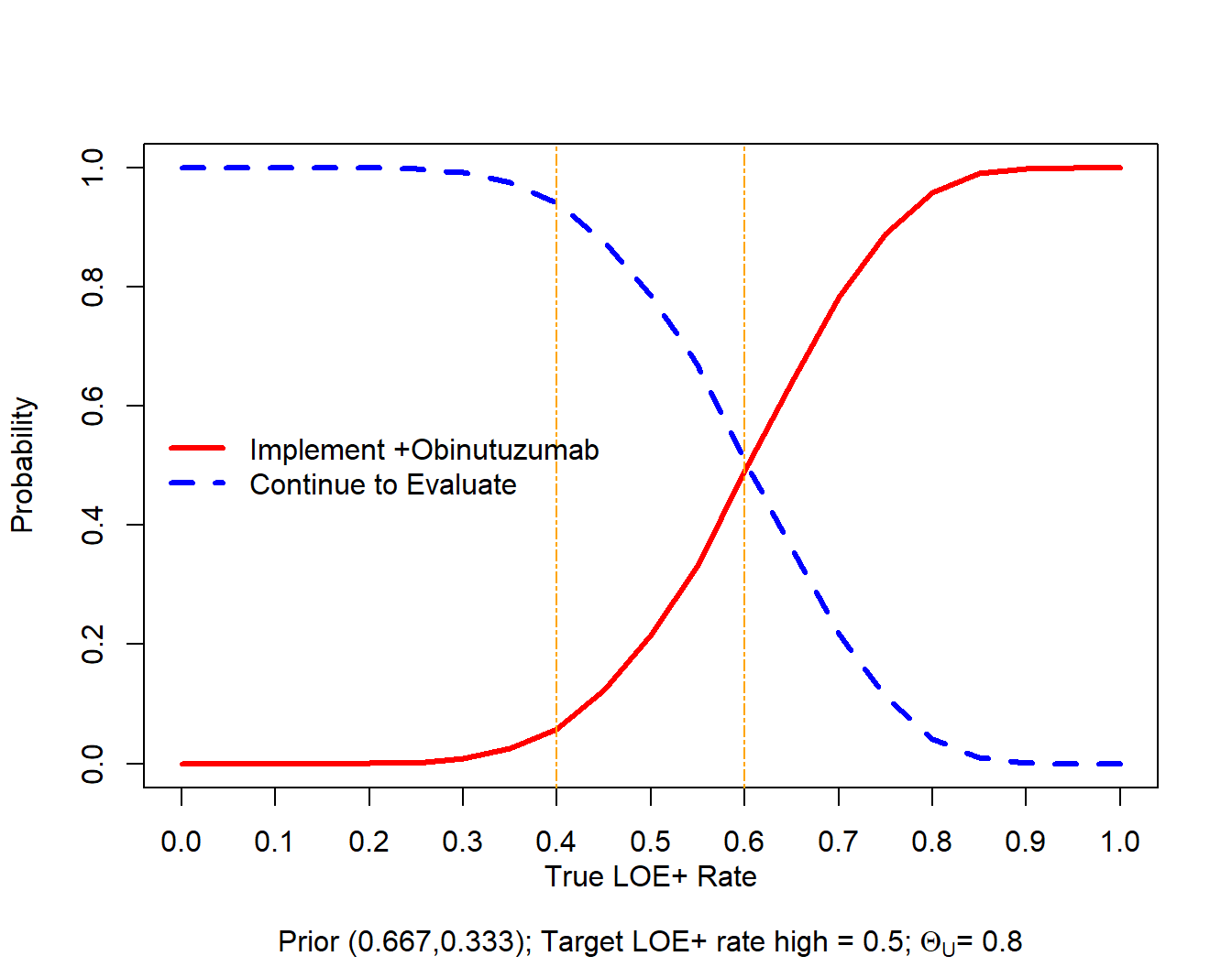
As an exemplary interpretation, if the true underlying LOE+ rate is 0.4 then the decision to proceed exclusively with obinutuzumab pretreatment will be taken in 5.8% of time. If instead the true underlying LOE+ rate is 0.6 then this decision would be taken only in 49.1% of time.
Final analysis with 41 patients
# total patient number at end of extension
nFin <- 41
The exact number of participants, with relevant loss of exposure, required to meet the criteria at subsequent evaluations will depend on the actual number of participants enrolled in each cohort and on the number of cohorts necessary to reach the end of the dose escalation. For these reasons the evaluation of the operating characteristics at the end of the dose escalation is done for a meaningful additional number of cohorts (9 cohorts), with constant cohort size (3 participants),
The question we then ask is how the posterior probabilities and operating characteristics change if we add 27 new patients to the trial. First, we again compute the posterior probabilities:
# posterior prob with final number of pts
postprob_nFin_h <-  postprob(x = c(0:nFin), n = nFin, p = target_h, parE = c(a_prior, b_prior))
postprob_nFin_l <-  postprob(x = c(0:nFin), n = nFin, p = target_l, parE = c(a_prior, b_prior))

tablepost_F <- as.data.frame(cbind(round(c(0:nFin), 0),
                                  round(postprob_nFin_h, 3),
                                  round((1 - postprob_nFin_l), 3)))
colnames(tablepost_F) <- c("n with LOE", "PP_h", "PP_l")
knitr::kable(tablepost_F)| n with LOE | PP_h | PP_l |
|---|---|---|
| 0 | 0.000 | 0.938 |
| 1 | 0.000 | 0.711 |
| 2 | 0.000 | 0.423 |
| 3 | 0.000 | 0.199 |
| 4 | 0.000 | 0.076 |
| 5 | 0.000 | 0.024 |
| 6 | 0.000 | 0.006 |
| 7 | 0.000 | 0.001 |
| 8 | 0.000 | 0.000 |
| 9 | 0.000 | 0.000 |
| 10 | 0.000 | 0.000 |
| 11 | 0.002 | 0.000 |
| 12 | 0.004 | 0.000 |
| 13 | 0.010 | 0.000 |
| 14 | 0.023 | 0.000 |
| 15 | 0.047 | 0.000 |
| 16 | 0.088 | 0.000 |
| 17 | 0.149 | 0.000 |
| 18 | 0.233 | 0.000 |
| 19 | 0.339 | 0.000 |
| 20 | 0.459 | 0.000 |
| 21 | 0.582 | 0.000 |
| 22 | 0.698 | 0.000 |
| 23 | 0.797 | 0.000 |
| 24 | 0.874 | 0.000 |
| 25 | 0.928 | 0.000 |
| 26 | 0.962 | 0.000 |
| 27 | 0.982 | 0.000 |
| 28 | 0.992 | 0.000 |
| 29 | 0.997 | 0.000 |
| 30 | 0.999 | 0.000 |
| 31 | 1.000 | 0.000 |
| 32 | 1.000 | 0.000 |
| 33 | 1.000 | 0.000 |
| 34 | 1.000 | 0.000 |
| 35 | 1.000 | 0.000 |
| 36 | 1.000 | 0.000 |
| 37 | 1.000 | 0.000 |
| 38 | 1.000 | 0.000 |
| 39 | 1.000 | 0.000 |
| 40 | 1.000 | 0.000 |
| 41 | 1.000 | 0.000 |
So as an illustration, at the final analysis after 41 patients we need to observe 24 or more participants with relevant loss of exposure to have a posterior probability equal or higher than 0.8 (\(\theta_U = 0.8\)) that the true LOE+ rate is \(\ge 0.5\).
We again first define a function that simulates trials with the given decision rule, including the decision to evaluate expansion cohorts both with and without obinutuzumab (see Section 2). At the end of the dose escalation, if the above criteria have not yet been met and, at the same time, there is low confidence (<70% confidence level) that the true underlying LOE+ rate is less than 5%, the expansion cohorts at the OBD with and without obinutuzumab will be evaluated.
myocpostF <-  function(p0, p1, a_prior, b_prior, myN, mytU, mytL, nn, nsim = 10 ^ 4){
  pgrid <- seq(from = 0, to = 1, by = 0.05)

  Probs <- expand.grid("nnF" = myN, "tU" = mytU, "tL" = mytL, "p" = pgrid)
  resProbs <- data.frame(matrix(NA, ncol = 3, nrow = nrow(Probs)) )
  colnames(resProbs) <- c("goProbs", "stopProbs", "greyProbs")

  for (parRun in seq_len(nrow(Probs))){
    auxpar <- Probs[parRun, ]
    thisOc <- ocPostprob(p = auxpar$p,
                         p0 = p0,
                         p1 = p1,
                         tL = auxpar$tL,
                         tU = auxpar$tU,
                         parE = c(a_prior, b_prior),
                         ns = nsim,
                         nr = FALSE,
                         nn = nn,
                         nnF = myN,
                         d = NULL)$oc
    resProbs[parRun, ] <- thisOc[ , c("PrEfficacy", "PrFutility", "PrGrayZone")]

  }
  TotProbs <- cbind(Probs, resProbs)
  return (TotProbs)
}
Then we again simulate 10^{4} trials to evaluate the operating characteristics:
set.seed(1234)
TotProbsB <- myocpostF(p0 = target_l, p1 = target_h, a_prior = a_prior, b_prior = b_prior,
                       myN = nFin, mytU = theta_h, mytL = theta_l,
                       nn = seq(from = n1i, to = nFin, by = 3),
                       nsim = nsim)
TotProbsB
nnF tU tL p goProbs stopProbs greyProbs
1 41 0.8 0.7 0.00 0.0000 1.0000 0.0000
2 41 0.8 0.7 0.05 0.0000 0.3857 0.6143
3 41 0.8 0.7 0.10 0.0000 0.0714 0.9286
4 41 0.8 0.7 0.15 0.0001 0.0105 0.9894
5 41 0.8 0.7 0.20 0.0004 0.0018 0.9978
6 41 0.8 0.7 0.25 0.0026 0.0001 0.9973
7 41 0.8 0.7 0.30 0.0129 0.0000 0.9871
8 41 0.8 0.7 0.35 0.0383 0.0000 0.9617
9 41 0.8 0.7 0.40 0.1104 0.0000 0.8896
10 41 0.8 0.7 0.45 0.2309 0.0000 0.7691
11 41 0.8 0.7 0.50 0.4125 0.0000 0.5875
12 41 0.8 0.7 0.55 0.6400 0.0000 0.3600
13 41 0.8 0.7 0.60 0.8170 0.0000 0.1830
14 41 0.8 0.7 0.65 0.9356 0.0000 0.0644
15 41 0.8 0.7 0.70 0.9849 0.0000 0.0151
16 41 0.8 0.7 0.75 0.9982 0.0000 0.0018
17 41 0.8 0.7 0.80 0.9999 0.0000 0.0001
18 41 0.8 0.7 0.85 1.0000 0.0000 0.0000
19 41 0.8 0.7 0.90 1.0000 0.0000 0.0000
20 41 0.8 0.7 0.95 1.0000 0.0000 0.0000
21 41 0.8 0.7 1.00 1.0000 0.0000 0.0000Now plot these operating characteristics again against the true assumed LOE+ rate:
matplot(TotProbsB$p, TotProbsB[, c("goProbs", "greyProbs", "stopProbs")],
        xlab = '', xaxt = "n", ylab = 'Probability', type= "l",
        col = c("red", "grey", "green"), lty = 1:3, lwd = 2)
at <- seq(0, 1, by = 0.1)
axis(side = 1, at = at)
abline(v = target_h, lty = 6, col = "red")
abline(v = target_l, lty = 6, col = "green")
legend ("right", c("Implement +Obinutuzumab", "Evaluate +/-Obinutuzumab", "Continue -Obinutuzumab"),
        col = c("red", "grey", "green"), lty = c(1, 2, 3), bty = "n")
title(sub = substitute(paste("Prior (", a, "," , b, "); ", "Target LOE+ rate: high =", h,
                             ", low =", l, "; ", Theta[U], "= " , theta_h, ", ", Theta[L], "= ",
                             theta_l), list(a = a_prior, b = b_prior, h = target_h, l = target_l,
                                            theta_h = theta_h, theta_l = theta_l)))
mtext(side = 1, 'True LOE+ Rate', line = 2) 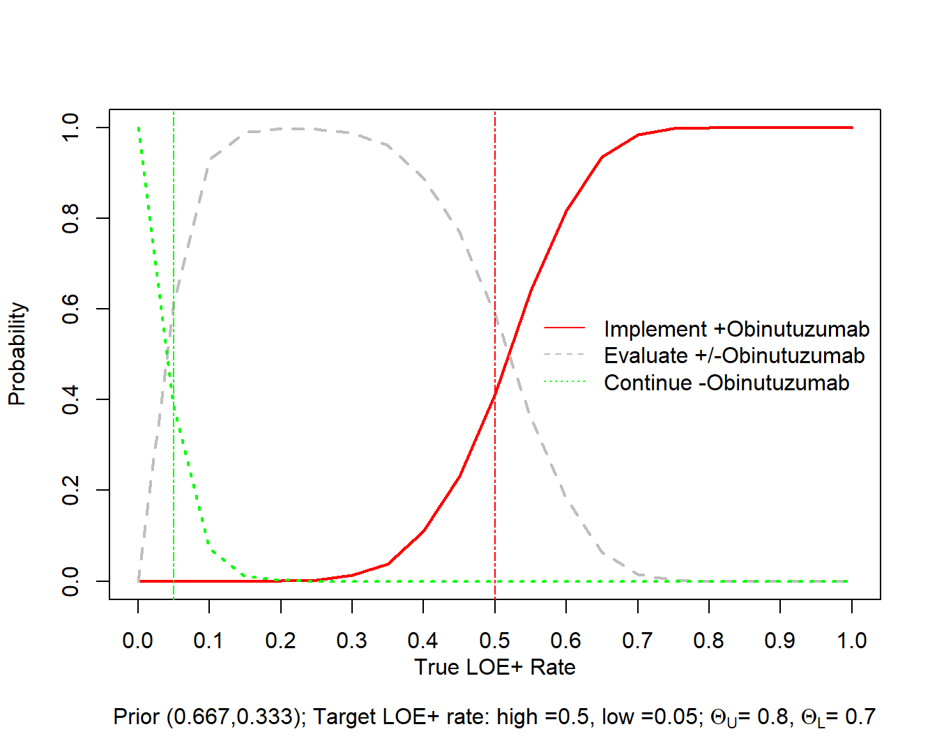
As an exemplary interpretation, if the true underlying LOE+ rate is 0.4 then the decision to proceed exclusively with obinutuzumab pretreatment will be taken in 11.0% of time. If instead the true underlying LOE+ rate is 0.6 then this decision would be taken only in 81.7% of time.
If the true underlying LOE+ rate is \(\le 0.05\) then the decision to proceed without obinutuzumab pre-treatment at the end of the trial will be taken in 38.6% of the times.