# Load bpp and rpact
library(bpp)
library(rpact)JACOB: update after interim if no prior had been specified
Setup
This is a recap of a trial that was performed. Numbers below are not everywhere exactly as in the trial, but that does not alter the story of what happened.
The trial
JACOB was a double-blind, placebo-controlled, randomised, multicentre, phase 3 trial in patients aged 18 years or older with HER2-positive metastatic gastric or gastro-oesophageal junction cancer. The treatments compared were Pertuzumab + Trastuzumab + chemotherapy vs. Placebo + Trastuzumab + chemotherapy. The primary endpoint was OS. Results have been reported here.
Design stage
Specifications of pivotal Phase 3 trial
We specify all the quantities of the pivotal trial, with explanations following below:
# specifications of JACOB
alpha <- 0.05
beta <- 0.2
hr <- 15 / 19.3
info <- 0.7

design <- getDesignGroupSequential(sided = 2, alpha = alpha, beta = beta,
                                   informationRates = c(info, 1),
                                   typeOfDesign = "asOF")
sampleSize <- getSampleSizeSurvival(design = design, hazardRatio = hr)

# number of events
nevents <- ceiling(as.vector(sampleSize$eventsPerStage))
nevents
[1] 352 502# MDDs
hrMDD <- sampleSize$criticalValuesEffectScaleLower
# efficacy boundary --> chosen based on the assumed local significance level
mdd_interim <- hrMDD[1, 1]
mdd_interim[1] 0.770872# MDD at final
mdd_final <- hrMDD[2, 1]
mdd_final[1] 0.8364363The assumptions for JACOB were:
- Two-sided significance level of \(\alpha = 0.05\).
- 1(treatment):1(control) randomization.
- 80% power to detect an overall hazard ratio of 0.777 using a standard log-rank test. This requires 502 OS events.
- The minimal detectable difference amounts to 0.771 at the efficacy interim after 70% of total information (corresponding to 352 events) and 0.836 at the final analysis.
Specification of prior
At the trial design stage there was no Phase 2 data or other external evidence available to inform a prior distribution. Therefore, no formal DDCP computation was done for JACOB, implying that no prior was specified. Instead, the PTS value at design stage of this trial was set to 0.75 and determined as follows:
- Take generic oncology Phase 3 PTS of 0.65.
- Increase this qualitatively for the following two reasons:
- Good results for Trastuzumab in same indication (TOGA trial).
- Good results for Pertuzumab + Trastuzumab in metastatic breast cancer (CLEOPATRA trial).
- Optimism based on increased assay sensitivity and capped enrollment of subgroup of Japanese patients who showed less benefit in TOGA.
Interim analysis
After not stopping the trial at the efficacy interim analysis after 70% of information it was clear to the broader team that DDCP (and therefore PTS) now should be reduced. Given that there was no prior data and therefore no prior DDCP calculation all PTS calculations were based on generic guidelines. So the question was by how much to reduce PTS?
Reverse-engineer a prior
One approach to inform how much to reduce PTS after the interim is to:
- Backengineer a Normal prior that corresponds to a DDCP of 75%.
- Quantify the change in DDCP after not stopping at the interim using this prior.
How to backengineer a Normal prior is described in this tutorial.
To derive the number of events \(d_0\) the Phase 2 data should correspond to for JACOB we simply consider a few scenarios as follows:
# determine number of events the prior knowledge should be worth of
pts2 <- 0.75
n0 <- c(25, 50, 100, 200)

# assume 1:1 randomization
propA0 <- 0.5
fac0 <- (propA0 * (1 - propA0)) ^ (-1)
sd0 <- sqrt(fac0 / n0)

# standard error of effect estimate at final analysis
propA <- 0.5
fac <- (propA * (1 - propA)) ^ (-1)
finalSE <- sqrt(fac / nevents[2])

# MDD on log-scale --> success criteria
successmean <- log(mdd_final)

# now find the prior means that correspond to this choice of pts2 and n0
delta0 <- successmean - qnorm(pts2) * sqrt(finalSE ^ 2 + sd0 ^ 2)

# prior hazard ratios
exp(delta0)
[1] 0.6344244 0.6847820 0.7215676 0.7472135The fewer prior events we assume the wider the prior density gets. This implies that the prior mean needs to be further away from the null hazard ratio of 1 to still give an initial DDCP of 75%. The priors look as follows:
xli <- log(c(0.35, 1.6))
yli <- c(-0.1, 2.9)
par(las = 1, mar = c(9, 5, 2, 1), mfrow = c(1, 1))
plot(0, 0, type = "n", xlim = xli, ylim = yli, xlab = "", ylab = "density",
     main = "Normal prior densities")
basicPlot(leg = FALSE, IntEffBoundary = NA, IntFutBoundary = NA, successmean = NA, priormean = NA)
segments(log(hrMDD), 0, log(hrMDD), 3, col = "brown", lwd = 4, lty = 2)
legend(-0.6, 2, "MDDs", lwd = 4, lty = 2, bty = "n", col = "brown")

# now add prior densities and corresponding DDCP values
thetas <- seq(0.3, 2.7, by = 0.01)
lthetas <- log(thetas)
for (i in 1:length(n0)){lines(lthetas, dnorm(lthetas, mean = delta0[i], sd = sqrt(fac0 / n0[i])),
                     col = i + 1, lwd = 4, lty = 1)}
legend("topleft", legend = paste(n0, " / ", disp(exp(delta0), 3)), col = 1 + 1:length(n0),
       lwd = 4, lty = 1, title = "Number of prior events and hazard ratios:", bty = "n")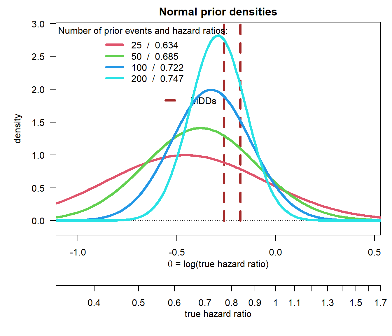
We can verify the computations:
bpp(prior = "normal", successmean = successmean, finalSE = finalSE,
    priormean = delta0, priorsigma = sd0)
[1] 0.75 0.75 0.75 0.75Now that we have defined a range of priors we can compute the drop in DDCP after not stopping at the efficacy interim, following the steps in the tutorial for interim updates for a time-to-event endpoint.
# compute DDCP after interim analysis for efficacy
# loop through all prior means
ddcp_interim <- rep(NA, length(n0))
for (i in 1:length(n0)){
  bpp_i <- bpp_1interim_t2e(prior = "normal", successHR = mdd_final, d = nevents,
                          IntEffBoundary = mdd_interim, IntFutBoundary = Inf, IntFixHR = 1,
                          priorHR = exp(delta0[i]), propA = 0.5, thetas = thetas,
                          priorsigma = sd0[i])
  ddcp_interim[i] <- bpp_i$"BPP after not stopping at interim interval"
}
ddcp_interim
[1] 0.2212007 0.2870107 0.3585434 0.4272722Let us wrap up the results:
| prior n | prior hazard ratio | initial DDCP | DDCP after interim | DDCP decrease |
|---|---|---|---|---|
| 25 | 0.634 | 0.75 | 0.221 | 0.529 |
| 50 | 0.685 | 0.75 | 0.287 | 0.463 |
| 100 | 0.722 | 0.75 | 0.359 | 0.391 |
| 200 | 0.747 | 0.75 | 0.427 | 0.323 |
The key conclusions by the team after this analysis were:
- The DDCP drop after interim decreases with increasing prior knowledge. This is plausible, as we have more prior data that we need to “overwhelm” with the trial.
- It appeared reasonable to assume that DDCP after not stopping at the interim is in the range of 30-50%.
- Using the pessimistic prior would not have relevantly changed that conclusion.