# Load bpp
library(bpp)

# load rpact
library(rpact)

# axis limits for plots
xli <- c(-1.1, 0.5)
yli <- c(-0.1, 2.7)Compute assurance at the design stage of a clinical trial: time-to-event endpoint
Purpose
This document provides code to compute assurance at the design stage of a clinical trial for a time-to-event primary endpoint. It thereby follows the computations in Rufibach et al. (2016), although with different numbers. All the references below to sections, figures, or tables are with respect to that paper.
We have designing a Phase 3 trial in mind, but the concepts are equally well applicable when designing a Phase 2 trial. In the latter case, the success criterion might be somewhat different.
Setup
Load packages:
Our trial of interest
We assume that we plan a 1:1 randomized trial for a time-to-event endpoint, so the effect measure we are interested in is the hazard ratio. Since we want to rely on a normally distributed test statistic all computations below implicitly happen on the scale of the log hazard ratio (which can be sufficiently well approximated through a Normal distribution). We further assume the trial will have one interim analysis after 50% of information. We start with defining the parameters of this pivotal trial:
# ---------------------------------------------------
# specifications of the pivotal trial
# ---------------------------------------------------

# set up a group-sequential design with an interim after 50% of information
# significance levels at final analysis
design <- getDesignGroupSequential(sided = 2, alpha = 0.05, beta = 0.2,
                                   informationRates = c(0.5, 1),
                                   typeOfDesign = "asOF")

# number of events needed
sampleSize <- getSampleSizeSurvival(design = design, hazardRatio = 0.75)
nevents <- ceiling(sampleSize$maxNumberOfEvents)
nevents
[1] 381# MDD at final
hrMDD <- sampleSize$criticalValuesEffectScaleLower[2, 1]
hrMDD[1] 0.8172823Define the prior distribution
As a next step we define the parameters of the prior density \(q(\theta)\), see Sections 4.1 and 4.2 in Rufibach et al. (2016). For a discussion of aspects of prior choice also see the tutorial on choice of prior.
Normal prior
# ----------------------------------
# mean and sd of Normal prior:
# ----------------------------------
hr0 <- 0.7

# Normal prior corresponding to information of 50 events in 1:1 randomized trial
sd0 <- sqrt(4 / 50)
The above prior could e.g. result from a Phase 2 trial with observed hazard ratio of 0.7 which we chose not to attenuate. The prior is centered at \(\theta_{prio} = \log(0.7)\). The resulting density function is depicted as red line in the figure below.
To better understand the properties of this prior we can compute a few probabilities of interest:
lims <- c(0.5, 1)
pnorm1 <- pnorm(log(lims[1]), mean = log(hr0), sd = sd0)
pnorm2 <- 1 - pnorm(log(lims[2]), mean = log(hr0), sd = sd0)
c(pnorm1, pnorm2)
[1] 0.1171001 0.1036479So the probability for the hazard ratio to be above 1 or below 0.5 amounts to 0.12 and 0.10, respectively. The prior thus allows for a 10% probability that the treatment effect may be on the harmful side.
# ----------------------------------
# parameters of pessimistic, or flat, prior:
# ----------------------------------
hr0flat <- 0.75
width1 <- 0.5
height1 <- 1
The above code specifies a more pessimistic alternative prior, see this tutorial for details on how to specify such a prior. This may potentially more accurately reflect the (absence of) knowledge about the treatment effect at the design stage or could be used as a kind of sensitivity analysis. Such a prior has e.g. been used when quantifying the success probability at the design stage in the MIRROS case study.
To specify a pessimistic prior we retain the lower tail of the Normal prior above but move the upper tail slightly to the right, allowing for a plateau in the center of the distribution. To compute the probabilities to be below 0 or above 1 we have to integrate over the density function of the pessimistic prior. The function for this density is available in the package bpp.
flat1 <- integrate(dUniformNormalTails, lower = -Inf, upper = log(lims[1]),
                   mu = log(hr0flat), width = width1, height = height1)$value
flat2 <- integrate(dUniformNormalTails, lower = log(lims[2]), upper = Inf,
                   mu = log(hr0flat), width = width1, height = height1)$value
c(flat1, flat2)
[1] 0.1089380 0.2125409This leads to a 21% probability for the true hazard ratio to exceed 1. The red line in the figure below illustrates this alternative prior.
par(las = 1, mar = c(9, 5, 2, 1), mfrow = c(1, 1))
plot(0, 0, type = "n", xlim = xli, ylim = yli, xlab = "", ylab = "density",
     main = "")
title(expression("Normal and pessimistic prior density for "*theta), line = 0.7)
basicPlot(leg = FALSE, IntEffBoundary = NA, IntFutBoundary = NA, successmean = NA,
          priormean = NA)

# grid to compute densities on
thetas <- seq(0.3, 2.7, by = 0.01)
lthetas <- log(thetas)

lines(lthetas, dnorm(lthetas, mean = log(hr0), sd = sd0), col = 2, lwd = 2)
lines(lthetas, dUniformNormalTails(lthetas, mu = log(hr0flat),
                                  width = width1, height = height1), lwd = 2, col = 3)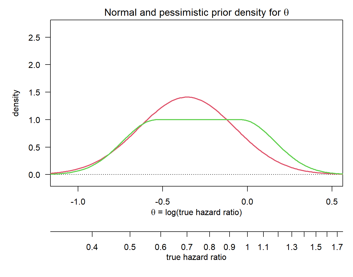
DDCP at the beginning of the trial
Having specified one or more priors together with the details of the trial of interest we can now quite easily compute the corresponding DDCP values.
# ----------------------------------
# Normal prior:
# ----------------------------------
bpp0 <- bpp_t2e(prior = "normal", successHR = hrMDD, d = nevents,
                priorHR = hr0, priorsigma = sd0)

# ----------------------------------
# pessimistic prior:
# ----------------------------------
bpp0_1 <- bpp_t2e(prior = "flat", successHR = hrMDD, d = nevents,
                  priorHR = hr0flat, width = width1, height = height1)

c(bpp0, bpp0_1)
[1] 0.6966965 0.5858342Note that the arguments for bpp differ, depending on which prior you want to compute DDCP for. We find that based on our priors and the specifications for the trial of interest we get values of 0.70 and 0.59. These are our BBP values at the design stage of the trial.
References
Rufibach, K., P. Jordan, and M. Abt. 2016. “Sequentially updating the likelihood of success of a Phase 3 pivotal time-to-event trial based on interim analyses or external information.” J Biopharm Stat 26 (2): 191–201. http://dx.doi.org/10.1080/10543406.2014.972508.