Methodology, Collaboration, and Outreach Group, PD DSS, Roche Basel
Published
Invalid Date
Purpose
This tutorial illustrates the dependence of DDCP on prior variability.
Setup
We assume that DDCP at the design stage has already been computed, as described in the corresponding tutorial.
DDCP and variability of the prior
DDCP is a function that depends on
the success criterion of the trial we want to compute DDCP for: this could be the MDD (corresponding to statistical significance), minimum TPP or target efficacy threshold,
the standard error of the estimate of the effect at the analysis of interest (interim or final) of the pivotal trial: this depends on the variability of the endpoint and the design of the trial of interest,
the specifications of the prior, e.g.
mean and standard error for the log(hazard ratio),
means and standard errors of mean(endpoint) for the active and control treatment for a continuous endpoint,
\(\beta\)-distribution parameters for the active and control treatment for a binary endpoint. If the prior is derived from an early phase trial, the latter is inversely proportional to the prior sample size.
It is important to note that DDCP of the pivotal trial depends on prior variability contingent on the location of the prior. To illustrate that we use again the scenario in the above linked tutorial. The MDD is at 0.483, 0.726, 0.814.
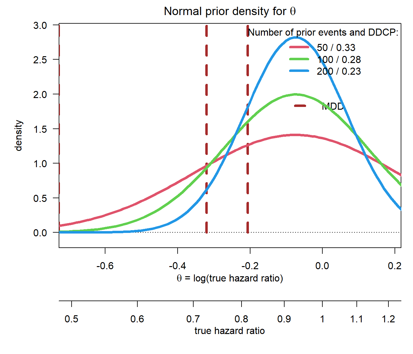
First, let us keep the prior mean from the above tutorial which is with a value of 0.93 located to the left of the MDD (i.e. since we are looking at the hazard ratio the prior effect is larger than the MDD) and vary the sample size:
par(las =1, mar =c(9, 5, 2, 1), mfrow =c(1, 1))xli <-log(c(0.5, 1.2))yli <-c(-0.1, 2.9)plot(0, 0, type ="n", xlim = xli, ylim = yli, xlab ="", ylab ="density", main =expression("Normal prior density for "*theta))basicPlot(leg =FALSE, IntEffBoundary =NA, IntFutBoundary =NA, successmean =NA, priormean =NA)segments(log(hrMDD), 0, log(hrMDD), 3, col ="brown", lwd =4, lty =2)legend(-0.1, 2, "MDD", lwd =4, lty =2, bty ="n", col ="brown")# now add prior densities and corresponding DDCP valuesthetas <-seq(-1.2, 1, by =0.01)n <-c(50, 100, 200)priorsigma <-sqrt(4/ n)bpps <-bpp(prior ="normal", successmean = successmean, finalSE = finalSE, priormean = priormean, priorsigma = priorsigma)m <-length(n)for (i in1:m){lines(thetas, dnorm(thetas, mean = priormean, sd =sqrt(4/ n[i])), col = i +1, lwd =4, lty =1)}legend("topright", legend =paste(n[1:m], " / ", disp(bpps[1:m], 2), sep =""), col =1+1:m, lwd =4, lty =1, title ="Number of prior events and DDCP:", bty ="n")
Of course, with increasing sample size the prior variability is decreasing. Since the prior mean corresponds to an effect that is better than the MDD increasing the sample size and therewith the precision for the prior implies that DDCP also increases as a function of prior sample size.
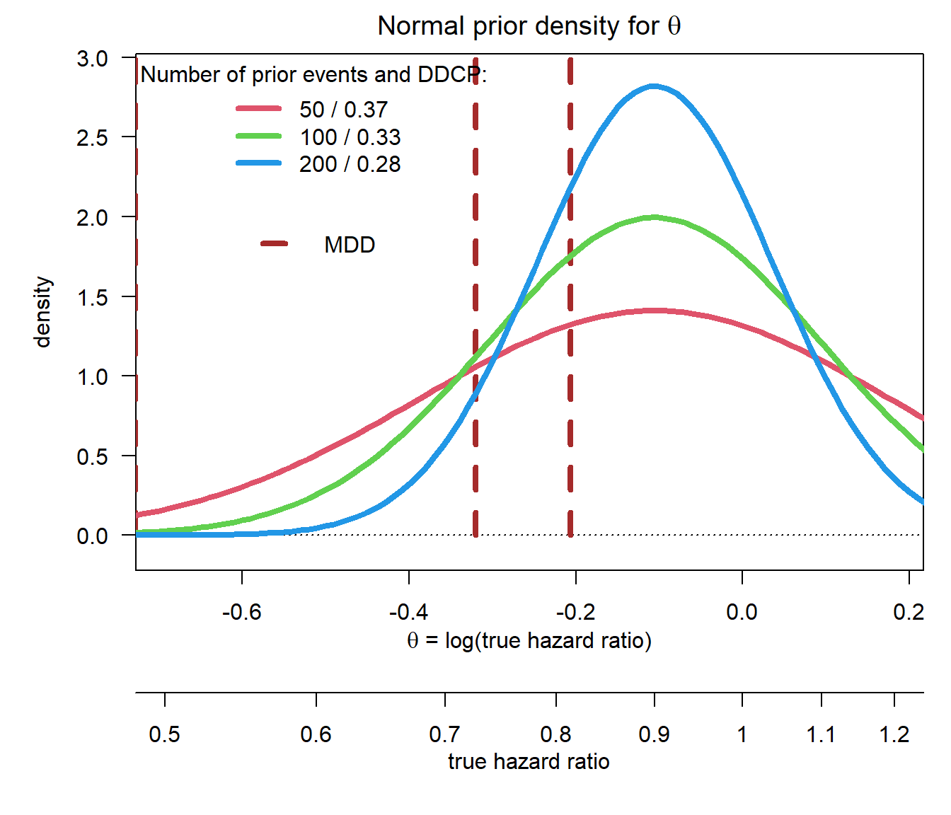
Now, let us assume the prior mean is with a value of -0.11 to the right of the MDD, i.e. corresponding to a smaller effect than the MDD:
par(las =1, mar =c(9, 5, 2, 1), mfrow =c(1, 1))plot(0, 0, type ="n", xlim = xli, ylim = yli, xlab ="", ylab ="density", main =expression("Normal prior density for "*theta))basicPlot(leg =FALSE, IntEffBoundary =NA, IntFutBoundary =NA, successmean =NA, priormean =NA)segments(log(hrMDD), 0, log(hrMDD), 3, col ="brown", lwd =4, lty =2)legend(-0.6, 2, "MDD", lwd =4, lty =2, bty ="n", col ="brown")# now add prior densities and corresponding DDCP valuespriormean <-log(0.9)bpps <-bpp(prior ="normal", successmean = successmean, finalSE = finalSE, priormean = priormean, priorsigma = priorsigma)for (i in1:m){lines(thetas, dnorm(thetas, mean = priormean, sd =sqrt(4/ n[i])), col = i +1, lwd =4, lty =1)}legend("topleft", legend =paste(n[1:m], " / ", disp(bpps[1:m], 2), sep =""), col =1+1:m, lwd =4, lty =1, title ="Number of prior events and DDCP:", bty ="n")
Now increasing the prior sample size leads to a decrease in DDCP, because the prior information is “worse” than the MDD.
Implications
These simple examples illustrate that one needs to be careful “tuning” the sample size of an early (Phase 2) trial based on DDCP of the potential pivotal trial.