# Load bpp and rpact
library(bpp)
Lade nötiges Paket: mvtnormlibrary(rpact)bpp and rpact installed as specified here.R code. Use the bpp help and the example Rmd files for guidance.\(\Rightarrow\) Good Luck!
bpp and rpact# Load bpp and rpact
library(bpp)Lade nötiges Paket: mvtnormlibrary(rpact)This exercise does hypothetical DDCP computations for the below trial. The setup was simplified to be able to concentrate on aspects relevant to DDCP computations.
Roche received accelerated approval for Triple-Negative Breast Cancer (TNBC) based on the IMpassion130 trial. As a post-marketing requirement (PMR) IMpassion131 was run, but that trial failed. As a consequence, it was evaluated whether yet another trial run by PDMA, IMpassion132, could stand in as PMR. To evaluate that feasibility it was of interest to update DDCP of IMpassion132 with the information from IMpassion 131, and that is what the task below is about.
Eventually, the TNBC label for Tecentriq based on IMpassion130 was withdrawn by Roche.
MO39193 (IMpassion132) is a phase III 1:1 randomized trial to investigate the efficacy and safety of Atezolizumab Plus Chemotherapy For Patients With Early Relapsing Recurrent (Inoperable Locally Advanced Or Metastatic) TNBC.
The primary endpoint of the trial is overall survival in PD-L1 positive patients.
The sample size section of the protocol states: The sample size is computed assuming that the trial gives 80% power for a hazard ratio of 0.7 and significance level of 0.05.
a) Compute the necessary number of events and the MDD for this trial.
Solution:
# adaptR code on https://pages.github.roche.com/adaptR/adaptR-tutorials/rpactSurvivalExamples.html
design <- getDesignGroupSequential(sided = 2, alpha = 0.05, beta = 0.2,
                                   informationRates = 1,
                                   typeOfDesign = "asOF")
sampleSize <- getSampleSizeSurvival(design = design, hazardRatio = 0.7)
summary(sampleSize)Fixed sample analysis, significance level 5% (two-sided). The results were calculated for a two-sample logrank test, H0: hazard ratio = 1, H1: hazard ratio = 0.7, control pi(2) = 0.2, event time = 12, accrual time = 12, accrual intensity = 120.2, power 80%.
| Stage | Fixed |
|---|---|
| Efficacy boundary (z-value scale) | 1.960 |
| Number of subjects | 1442.9 |
| Number of events | 246.8 |
| Analysis time | 18.000 |
| Expected study duration | 18.0 |
| Two-sided local significance level | 0.0500 |
| Lower efficacy boundary (t) | 0.779 |
| Upper efficacy boundary (t) | 1.283 |
Legend:
# number of events needed
nevents0 <- ceiling(sampleSize$maxNumberOfEvents)
nevents0
[1] 247# MDD
hrMDD <- sampleSize$criticalValuesEffectScaleLower[1, 1]
hrMDD[1] 0.7791696b) Now assume a Normal prior centered around a hazard ratio of 0.75 and worth 50 events (1:1 randomization). What is the DDCP at design stage?
Solution:
# ----------------------------------
# mean and sd of Normal prior:
# prior corresponding to information of 50 events in 1:1 randomized trial
# ----------------------------------
hr0 <- 0.75
n0 <- 50
sd0 <- sqrt(4 / n0)

# compute DDCP
bpp0 <- bpp_t2e(prior = "normal", successHR = hrMDD, d = nevents0,
                priorHR = hr0, priorsigma = sd0)
bpp0
[1] 0.5489551c) Now results of the related trial IMpassion131 become known: here, patients were randomized 2:1 and a hazard ratio of 1.12 was observed based on 120 events. How does DDCP change with this information?
Solution:
# ----------------------------------
# update the Normal prior with this information
# ----------------------------------
hr1 <- 1.12
nevents1 <- 120
propA1 <- 2 / 3
fac1 <- (propA1 * (1 - propA1)) ^ (-1)
se1 <- sqrt(fac1 / nevents1)
up1 <- NormalNormalPosterior(datamean = log(hr1), sigma = se1, n = 1, nu = log(hr0),
                             tau = sd0)

# specifications of posterior
exp(up1$postmean)
[1] 0.9854534up1$postsigma[1] 0.1597871# recompute DDCP
bpp1 <- bpp_t2e(prior = "normal", successHR = hrMDD, d = nevents0,
priorHR = exp(up1$postmean), priorsigma = up1$postsigma)
bpp1[1] 0.1251097So with this new information the posterior is centered at a hazard ratio of 0.985 and DDCP drops from 0.549 to 0.125.
d) Now assume that at trial onset there was little knowledge about the underlying effect, i.e. we assume that hazard ratios between 0.4 and 1.1 were equally likely. Specify such a prior and compute DDCP at the design stage.
Solution:
# ----------------------------------
# parameters of pessimistic, or flat, prior:
# ----------------------------------
ea <- 0.4
eb <- 1.1
a <- log(ea)
b <- log(eb)
width1 <- b - a
priormeanflat <- (a + b) / 2
height1 <- 0.7

# DDCP at design stage
bpp0_1 <- bpp_t2e(prior = "flat", successHR = hrMDD, d = nevents0,
                  priorHR = exp(priormeanflat), width = width1, height = height1)
bpp0_1
[1] 0.6126707The height of the pessimistic prior can be freely chosen as long as there is enough “area” left for the two tails, i.e. width \(\cdot\) height must be strictly \(<1\). See the tutorial on prior choice for a further discussion of this aspect. For the definition of the width we need to make sure we act on the log-scale, see also the tutorial on MIRROS.
e) Finally, plot the prior, the density of the external data, and the posterior for the Normal prior, as well as the density function of the pessimistic prior.
Solution:
par(las = 1, mar = c(9, 5, 2, 1), mfrow = c(1, 1), cex = 0.8)
leg <- c("prior", "IMpassion131 data", "posterior after IMpassion131", "pessimistic prior")
thetas <- seq(-2, 1, by = 0.01)

# ----------------------------------
# Normal prior:
# ----------------------------------
plot(0, 0, type = "n", xlim = log(c(0.3, 2)), ylim = c(0, 2.7), xlab = "", ylab = "density",
     main = "")
title(expression("Normal prior density and posteriors for "*theta), line = 0.7)
basicPlot(leg = FALSE, IntEffBoundary = NA, IntFutBoundary = NA, successmean = log(hrMDD),
          priormean = log(hr0))

# prior
lines(thetas, dnorm(thetas, mean = log(hr0), sd = sd0), col = 1, lwd = 2)

# data
lines(thetas, dnorm(thetas, mean = log(hr1), sd = se1), col = 2, lwd = 2)

# posterior
lines(thetas, dnorm(thetas, mean = up1$postmean, sd = up1$postsigma), col = 3, lwd = 2)

# pessimistic prior density
lines(thetas, dUniformNormalTails(thetas, mu = priormeanflat,
                                  width = width1, height = height1), lwd = 2, col = 4)

legend(-1.2, 2.7, leg, lty = 1, col = 1:4, bty = "n", lwd = 2)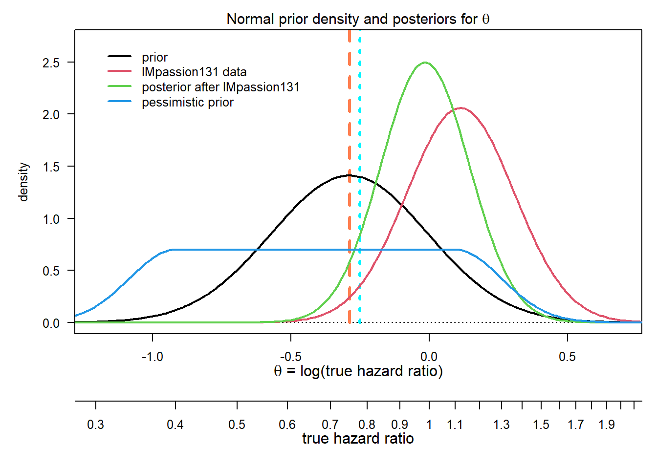
This exercise does hypothetical DDCP computations for the below trial. The setup was simplified to be able to concentrate on aspects relevant to DDCP computations.
GA28950 is a phase III 4:1 randomized trial to investigate the efficacy and safety of etrolizumab during inducation and maintenance in patients with moderate to severe active ulcerative colitis who are refractory to or intolerant of TNF inhibitors.
The primary endpoint of the blinded induction cohort is the proportion of patients in remission at Week 14.
The sample size section of the protocol states (slightly modified): Cohort 2 patients will be randomized in a 4:1 ratio to etrolizumab or placebo. This will provide 90% power to detect a 10% difference in remission rates at Week 14 between the etrolizumab and placebo arms, under the assumption of a placebo remission rate of 5% and a two-sided \(\chi^2\) test at the 5% significance level.
a) Compute sample size and MDD.
Solution:
# adaptR code on https://pages.github.roche.com/adaptR/adaptR-tutorials/rpactBinaryExamples.html
pi2 <- 0.05
delta <- 0.1
pi1 <- pi2 + delta

sampleSize <- getSampleSizeRates(pi2 = pi2, pi1 = pi1,
    sided = 2, alpha = 0.05, beta = 0.1,
    allocationRatioPlanned = 4)
summary(sampleSize)Fixed sample analysis, significance level 5% (two-sided). The results were calculated for a two-sample test for rates (normal approximation), H0: pi(1) - pi(2) = 0, H1: treatment rate pi(1) = 0.15, control rate pi(2) = 0.05, planned allocation ratio = 4, power 90%.
| Stage | Fixed |
|---|---|
| Efficacy boundary (z-value scale) | 1.960 |
| Number of subjects | 602.8 |
| Two-sided local significance level | 0.0500 |
| Lower efficacy boundary (t) | -0.031 |
| Upper efficacy boundary (t) | 0.059 |
Legend:
# sample size
n <- ceiling(sampleSize$maxNumberOfSubjects)
n
[1] 603# MDD
mdd <- sampleSize$criticalValuesEffectScaleUpper[1, 1]
mdd[1] 0.05915225b) Assuming that 0.05 in the control arm is the true remission proportion, what proportion in the intervention arm do we need to observe to get a 2-sided \(p\)-value of 0.05 in this trial?
Solution: We need to observe \(\pi_2 + \text{MDD} = 0.05 + 0.0591522 = 0.1091522.\)
c) Assume we want to be statistically significant at the final analysis, i.e. to beat the MDD. DDCP is the probability for this event, averaged over a prior distribution - write the formula for DDCP down.
Solution: Define the effect size \(\delta = \pi_1 - \pi_2\) and a prior density \(q(\delta)\). Then,
\[\text{DDCP} = \int_{-1}^1 P(\hat \delta \ge \text{MDD}) q(\delta) d \delta.\]
d) Write down the Normal approximation to the distribution of \(\delta\).
Solution: \[\hat \delta \sim N\Bigl(\delta, \text{SE}(\hat \delta)\Bigr)\]
with \(\text{SE}(\delta) = \sqrt{\hat \pi_1 \cdot (1 - \hat \pi_1) / n_1 + \hat \pi_2 \cdot (1 - \hat \pi_2) / n_2}\), where \(n_1\) and \(n_2\) are the sample sizes in each arm.
e) Now assume in a 1:1 randomized Phase 2 trial with 50 patients we observed 4 and 2 remissions. Based on this result construct a Normal prior for the response proportion difference. The standard error is computed assuming an overall proportion of \(\pi_0 = 0.07\). Plot this prior distribution.
Solution: 4 and 2 remissions give proportions of 0.16 and 0.08, and therefore a remission rate difference \(\delta\) of 0.08 which is worth 50 patients. The corresponding density \(q(\delta)\) is \(N(0.08, \sqrt{2 \cdot 0.07 \cdot (1 - 0.07) / 25}).\)
# prior definitions
n0 <- 50
pi0 <- 0.07
sd0 <- sqrt(2 * pi0 * (1 - pi0) / (n0 / 2))

# plot
par(las = 1, mar = c(4.5, 4.5, 2, 1))
thetas <- seq(-1, 1, by = 0.01)
plot(0, 0, type = "n", xlim = c(-0.1, 0.25), ylim = c(0, 7),
     xlab = expression("proportion difference "*delta), ylab = "density",
     main = "")
title(expression("Normal prior density "*delta), line = 0.7)

lines(thetas, dnorm(thetas, mean = pi0, sd = sd0), col = 2, lwd = 2)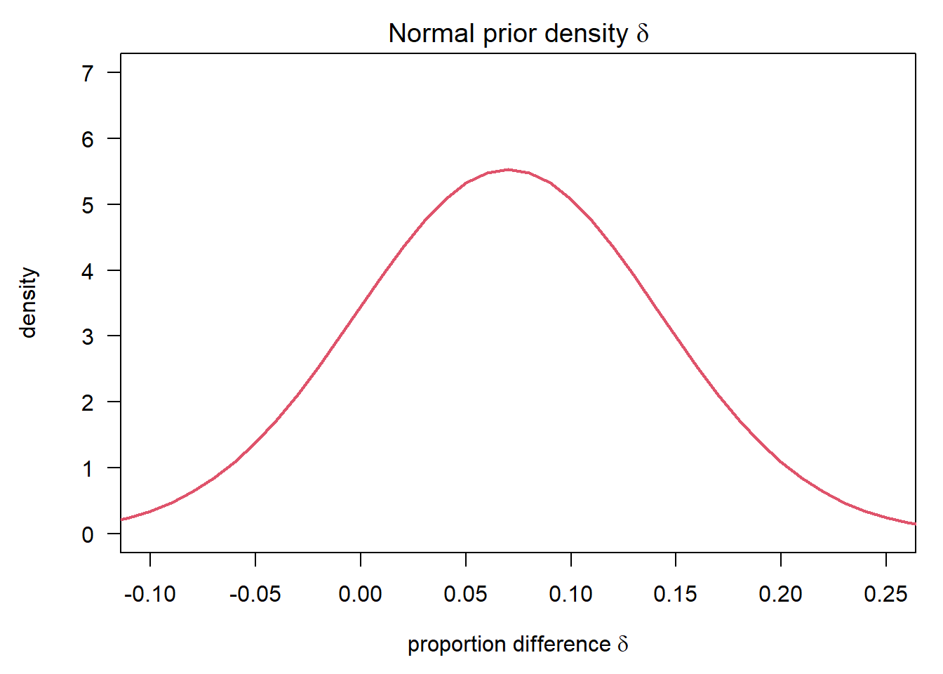
f) Now compute DDCP at the design stage using this prior.
Solution: The bpp package is built such that it always considers \(\le\). So we redefine accordingly and mirror all the above quantities.
# in computation of SE, account for the 4:1 randomization
bpp0 <- bpp_binary(prior = "normal", successdelta = mdd, pi1 = pi1, n1 = 4 * n / 5,
                   pi2 = pi2, n2 = n / 5, priormean = pi0, priorsigma = sd0)
bpp0
[1] 0.5563148The Normal approximation might not work terribly well for small sample sizes of the Phase 3 or when \(\pi_1, \pi_2\) are close to zero or one (as in this example). The usual rule-of-thumb is that the Normal approximation is accurate enough if the expected number of responders and non-responders in each arm is \(\ge 5\), i.e.
are all \(\geq 5\). This is met in this example still, as the sample size is quite large. However, if this rule-of-thumb is not met, exact results can be obtained by replacing the above integral through a sum over binomial probabilities. See the binary endpoint design tutorial for details.
This exercise does hypothetical DDCP computations for the above trial which was also discussed in the adaptR exercises. The setup below was simplified to be able to concentrate on aspects relevant to DDCP computations.
WN29922 is a phase III, multicenter, 1:1 randomized, double-blind, placebo-controlled, parallel-group, efficacy, and safety trial of gantenerumab in patients with early (prodromal to mild) Alzheimer's disease.
The primary endpoint of the trial is change from baseline (Day 1) to Week 104 in global outcome, as measured by the Clinical Dementia Rating - Sum of Boxes (CDR-SOB).
To cut the story short, the assumption was that for a continuous endpoint a sample size of approximately 500 patients for the trial has 80% power to detect a reduction in the change score from 2.5 to 1.75. The sample size calculation did not formally account for interim analyses but the protocol states that an interim analysis for efficacy and futility will be conducted after 50% of the targeted trial enrollment has been reached and that type I error control will be achieved by using O'Brien-Fleming boundaries approximated using the Lan-DeMets \(\alpha\)-spending method. The design specifications are as follows, just copying them over from the adaptR exercises to avoid hard-coding:
# Total sample size without inflation due to dropout
result <- getSampleSizeMeans(alternative = 2.5 * 0.3, stDev = 2.97,
                             sided = 2, alpha = 0.05, beta = 0.2)
design <- getDesignGroupSequential(sided = 1, alpha = 0.025, beta = 0.2,
    informationRates = c(0.5,1),
    typeOfDesign = "asOF",
    futilityBounds = 0, bindingFutility = FALSE)
resultGS <- getSampleSizeMeans(design, alternative = 2.5 * 0.3, stDev = 2.97) a) Assume that at the design stage, a prior which puts equal weight on a reduction of 0% up to 50% is chosen. Specify such a prior and plot it.
Solution:
If you look at the rpact output you find that everything is shifted to have 80% power to test \(H_0: \delta = 0\) vs. \(H_1: \delta = 0.3 * 2.5 = 0.75\). The MDD at the interim and final analysis is shown to be 1.124 and 0.524. Now, since bpp is always looking at \(\le\) we flip everything, i.e. we look at \(H_0: \delta = 0\) vs. \(H_1: \delta = -0.75\) with MDDs -1.124 and -0.524.
So we want a prior that is uniform from -1.25 (= 50% reduction) up to 0 (= 0% reduction).
# ----------------------------------
# parameters of pessimistic, or flat, prior:
# ----------------------------------

# center and width of the prior
# the height is a parameter that governs the tails and can be
# freely chosen, within limits such that we still get a density
priormeanflat <- 1.25 / 2
width1 <- 1.25
height1 <- 0.5

par(las = 1, mar = c(4.5, 4.5, 2, 1), mfrow = c(1, 1))
xli <- priormeanflat + width1 * c(-1, 1) * 1.2
yli <- c(0, 0.55)
plot(0, 0, type = "n", xlim = xli, ylim = yli,
     xlab = "reduction in change of points", ylab = "density",
     main = "Pessimistic prior density for reduction in change of points")
abline(h = 0, lty = 3)

# grid to compute densities on
thetas <- seq(min(xli), max(xli), by = diff(range(xli)) / 1000)

lines(thetas, dUniformNormalTails(thetas, mu = priormeanflat,
                                  width = width1, height = height1), lwd = 2, col = 3)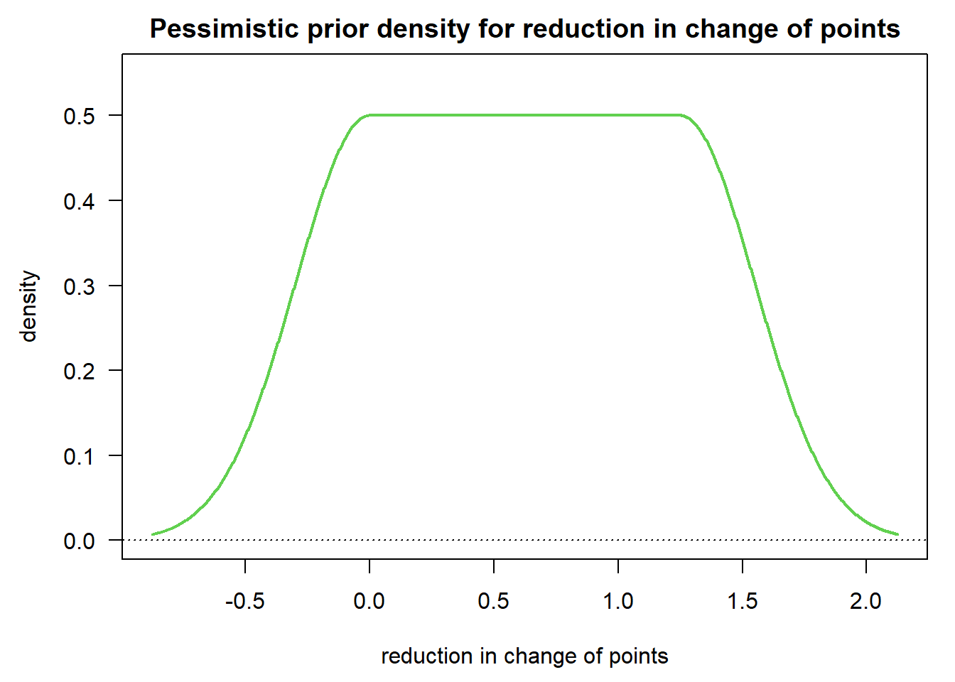
b) Now, assuming a standard deviation of 3 in each arm compute the DDCP at the design stage.
Solution:
successmean <- resultGS$criticalValuesEffectScale[2, 1]
successmean
[1] 0.5242053n_fin <- ceiling(resultGS$nFixed / 2) # number of patients at final analysis, per arm
n_fin[1] 248stDev <- 3
# DDCP at design stage
bpp0_1 <- bpp_continuous(prior = "flat", successmean = successmean, stDev = stDev,
n1 = n_fin, n2 = n_fin, priormean = priormeanflat,
width = width1, height = height1)
bpp0_1[1] 0.5503062c) Now assume that (unlike in the protocol) an interim for efficacy is performed after 50% of information, with MDD = -1.124. The trial does not stop at this interim, but the team does not know which estimate was observed. How does that change the team’s DDCP?
# standard error at interim
n_int <- n_fin / 2    # number of pts at interim, per arm

# efficacy boundary
effi <- 1.124

# futility boundary - no stop for futility
futi <- -Inf

# compute DDCP
bpp3_1_effi_only <- bpp_1interim_continuous(prior = "flat", successmean = successmean, stDev = stDev,
                               n1 = c(n_int, n_fin), n2 = c(n_int, n_fin),
                               IntEffBoundary = effi, IntFutBoundary = futi, IntFix = 1,
                               priormean = priormeanflat, propA = 0.5, thetas = thetas, width = width1,
                               height = height1)$"BPP after not stopping at interim interval"
bpp3_1_effi_only
[1] 0.3908396So DDCP drops from 0.550 to 0.391 after not stopping at this interim for efficacy.