# if you have not installed it yet first install probSuccess
if (1 == 0){install.packages("probSuccess", repos = "https://restst.gene.com/gran/current")}

# load probSuccess
library(probSuccess)
library(tidyverse)Compute assurance with the package probSuccess
Purpose
This document provides examples of computations that are possible with the package probSuccess, written by Paul Jordan and available here, with github repository here. Many of the computations that are documented in the tutorials can be done with probSuccess as well, but that package also offers additional possibilities. These are documented below. The entire documentation file written by Paul is available here.
Load package:
Multivariate continuous endpoints
External information, 2-dimensional endpoint, without prior
The endpoint is represented as a 2-dim vector: \(\vec{y}=(y_1,y_2)\).
- Critical value: \(\vec{y}_c = (12, 11)\)
- Endpoint: Difference to placebo.
- Sample-size of first study: \(N_{old}=30\)
- Sample-size of planned new study: \(N_{new} = 80\)
- Observed mean in a previous stud : \((\bar{y_1}, \bar{y_2}) =(11.6, 11.3)\).
- Observed covariance matrix: \(\mathbf{S}= \begin{bmatrix} \mathbf{9.3} & \mathbf{4.2}\\ \mathbf{4.2} & \mathbf{15.8}\\ \end{bmatrix}\)
COV   <- matrix(c(9.3, 4.2, 4.2, 15.8), ncol = 2)
M     <- c(11.6, 11.3)
PTSafterStudyMV(TPP = c(12, 11),Mean=M,N=30,nNew=80,Cov=COV,diffRef=TRUE)
[1] 0.2473748Adding a prior:
Let us assume that our previous knowledge on the 2-dimesional endpoint is represented by:
\[\mathcal{N}\left( \mu= \begin{bmatrix} 10\\ 10 \end{bmatrix}, \Sigma= \begin{bmatrix} \mathbf{20} & \mathbf{0}\\ \mathbf{0} & \mathbf{20}\\ \end{bmatrix} \right)\]
Sigma <- 20*diag(2)
PTSafterStudyMV(TPP=c(12,11),Mean=M,N=30,nNew=80,Cov=COV,diffRef=TRUE,
                ,prior=dmvnorm,mean=c(10,10),sigma=Sigma)
[1] 0.2208253Internal information
Let us consider the following example:
- Bivariate endpoint at the interim analysis (20 subjects).
- The means are differences to a reference group (
diffRef=TRUE). - the mean for endpoint I is \(11.2\) and the mean for endpoint II \(11.9\).
- The covariance matrix of the observations is:\(\mathbf{S}= \begin{bmatrix} \mathbf{9.3} & \mathbf{4.2}\\ \mathbf{4.2} & \mathbf{15.8}\\ \end{bmatrix}\)
- The cutpoint for success is \(11\) for either endpoint.
- Final analysis after 55 subjects.
- Prior on the endpoint: \(\mathcal{N}\left( \mu= \begin{bmatrix} 10\\ 10 \end{bmatrix}, \Sigma= \begin{bmatrix} \mathbf{50} & \mathbf{0}\\ \mathbf{0} & \mathbf{50}\\ \end{bmatrix} \right)\)
MeanIA <- c(11.2,11.9)
nIA    <- 20
nFinal <- 55
CovIA  <- matrix(c(9.2,3.1,3.1,15.8),ncol=2)
TPP    <- c(11,11)

PTSafterIAMV(TPP,type="value",MeanIA=MeanIA,IntIA=NULL,CovIA=CovIA,nIA=nIA
               ,nFinal=nFinal,diffRef=TRUE
               ,prior=dmvnorm,mean=c(10,10),sigma=50*diag(2))
[1] 0.5061063Now let us assume, that at the IA, there is only known (other specification equal):
- Mean I lies in the interval [10,12]
- Mean II lies in the interval [9,13]
IntIA <- IntIA <- rbind(c(10,12),c(9,13))
PTSafterIAMV(TPP=c(11,11),type="interval",MeanIA=NULL,IntIA=IntIA
               ,CovIA=CovIA,nIA=nIA,nFinal=nFinal,diffRef=TRUE,prior=dmvnorm
               ,mean=c(10,10),sigma=50*diag(2))
[1] 0.257443Survival analyses
The probability of success is defined as the probability to observe a hazard ratio less than a critical value in a trial with n events. The previous knowledge about the true hazard ratio \(\lambda\) is expressed in the original scale by a lognormal distribution with mean \(\mu\) and variance \(\sigma^2\).
PSsurvival(Mlambda=0.9,Slambda=0.04,Crit=0.814,n=630)[1] 0.1402306Examples for conditional and predictive power
The functions are based on the unified approach using the appropriate z-statistic (Proschan, Lan, and Wittes 2006). More details are given in the documentationto probSuccess.
Conditional power: Comparing two means
The example is taken from (Dmitrienko and Wang 2006) (page 2187). In the paper, alpha is one-sided.
meanT <- 9.2
sdT   <- 7.3
n1T   <- 11
n2T   <- 41

meanC <- 8.4
sdC   <- 6.4
n1C   <- 10
n2C   <- 41

CondPowerMeans(meanT=meanT, meanC=meanC, sdT=sdT, sdC=sdC, n1T=n1T, n1C=n1C, n2T=n2T, n2C=n2C,
               delta = 4, sigma=8.5, alpha = 0.2)
[1] 0.6948443Conditional power: Comparing two proportions
The example is taken from (Proschan, Lan, and Wittes 2006), Example 3.3. (page 50ff).
CondPowerRates(kT=24,kC=22,n1T=48,n1C=44,n2T=200,n2C=200,PT=0.45,PC=0.6)[1] 0.6567376assurance: Comparing two means
The example is taken from (Proschan, Lan, and Wittes 2006), Example 3.2.
delta  <- 2     ## expected difference between treatment and control
sigma  <- 5     ## expected SD of difference
n1T    <- 52
n1C    <- 50
n2T    <- 132
n2C    <- 132
diff   <- 1     ## observed treatment difference at interim analysis
s_pool <- 6.1   ## observed pooled standard error
The prior information is given a weight of ca. 10% compared to data at the end of the trial; therefore: \[\frac{1/\sigma_0^2} {1/\sigma_0^2 + 1} = 0.1 \rightarrow \sigma_0^2 = 9\]
sigma.0 <- 3

## Type I error one-sided: 0.025

PredPowerMeans(meanT=diff, meanC=0, sdT=s_pool, sdC=s_pool, n1T=n1T, n1C=n1C, n2T=n2T, n2C=n2C
                 ,delta.0 = delta, sigma=sigma ,sigma.0=sigma.0,alpha = 0.025)
[1] 0.3775832For \(\sigma_0^2 = 0\), the predictive power coincides with the conditional power:
PP <- PredPowerMeans(meanT=diff, meanC=0, sdT=s_pool, sdC=s_pool, n1T=n1T, n1C=n1C, n2T=n2T, n2C=n2C
               ,delta.0 = delta, sigma=sigma, sigma.0=0, alpha = 0.025)

print(PP)
[1] 0.7582574CP <- CondPowerMeans(meanT=diff, meanC=0, sdT=s_pool, sdC=s_pool, n1T=n1T, n1C=n1C, n2T=n2T, n2C=n2C
,delta = delta, sigma=sigma, alpha = 0.05) ## two-sided alpha!
print(CP)[1] 0.7582574Examples for Bayesian methods
Updating a prior distribution by the result of a previous study
Data from a previous pilot study (continuous and normally distributed endpoint):
- Observed mean: \(\bar{x}=11\)
- Observed standard deviation: \(\text{sd}(x)=4\)
- Number of observations: 8
As prior for the population mean \(\mu\), a generalized t-distribution with location \(\mu=8\), scale \(\sigma=2\) and \(\nu=1\) degrees of freedom is chosen:
Mean <- 11
SD   <- 4
N    <- 8

m_p  <- 8
sd_p <- 2
nu_p <- 1

mu             <- seq(4,15,0.1)
prior          <- dT(mu,nu_p,m_p,sd_p)
post           <- updatePriorMean(mu,type="value",Mean=Mean,SD=SD,Int=NULL,N=N
                              ,diffRef=FALSE,prior=dT,nu=nu_p,m=m_p,s=sd_p)

Density <- c(prior,post)
Type    <- rep(c("prior","posterior"),each=length(mu))
mu      <- rep(mu,2)

PostDens <- data.frame(mu,Density,Type)
plotPost <- ggplot(PostDens,aes(x=mu,y=Density,col=Type)) + geom_line() +
                   geom_vline(xintercept=Mean,linetype="dashed",col="blue") +
                   annotate("text",x=Mean,y=0.025,label = expression(bar(x)==11),
                            hjust=0,col="blue")
print(plotPost)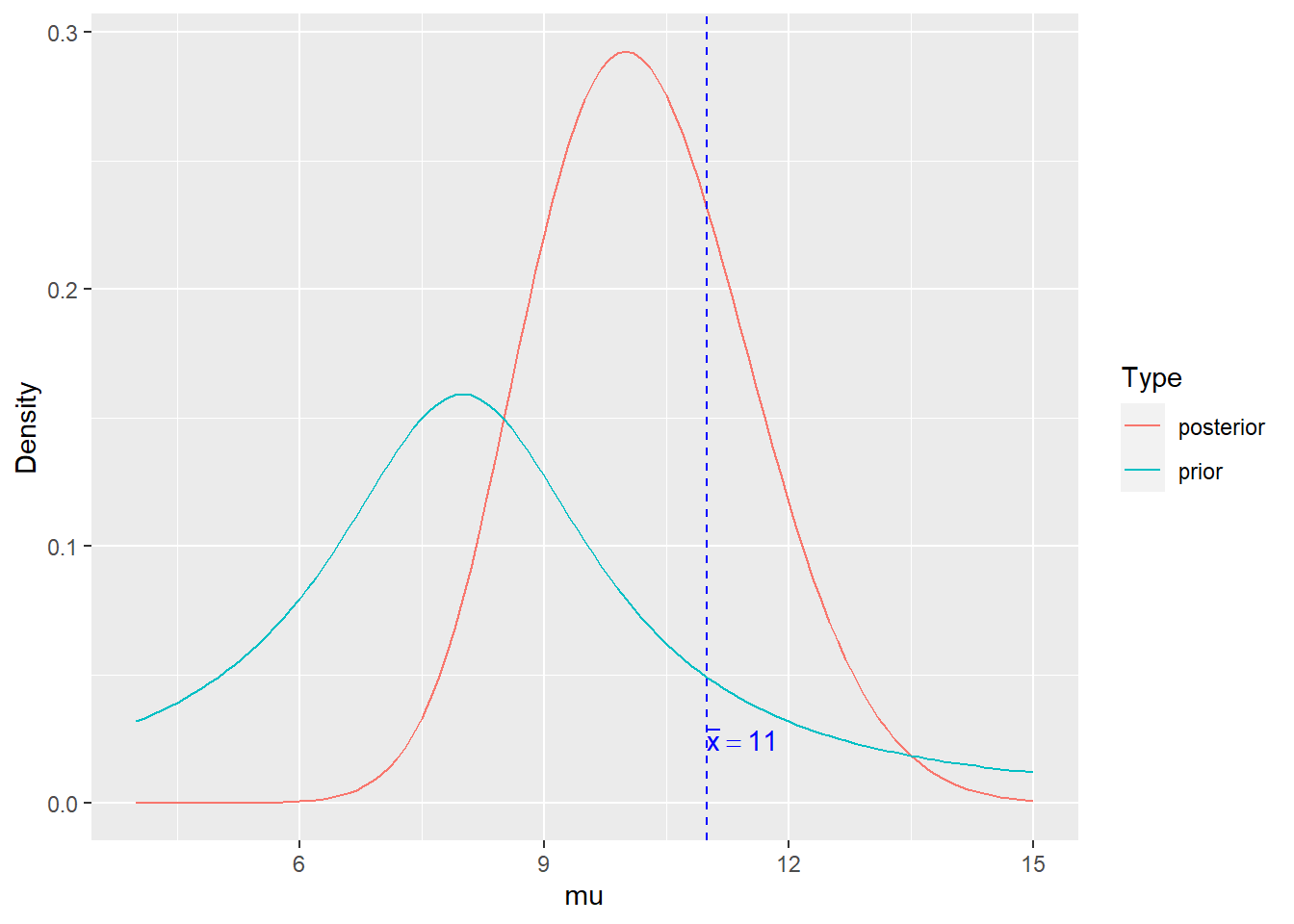
If instead of the mean, only an interval containing the mean is known: \(\bar{x} \in [0,9]\):
mu <- seq(-5,15,0.1)
prior          <- dT(mu,nu_p,m_p,sd_p)

post<- updatePriorMean(mu,type="interval",SD=2,Int=c(0,9),N=16
                      ,diffRef=TRUE,prior=dT,nu=2,m=11,s=10)

Density <- c(prior,post)
Type    <- rep(c("prior","posterior"),each=length(mu))
mu      <- rep(mu,2)

PostDens <- data.frame(mu,Density,Type)

plotPost <- ggplot(PostDens,aes(x=mu,y=Density,col=Type)) + geom_line() +
                   geom_vline(xintercept=Mean,linetype="dashed",col="blue")

print(plotPost)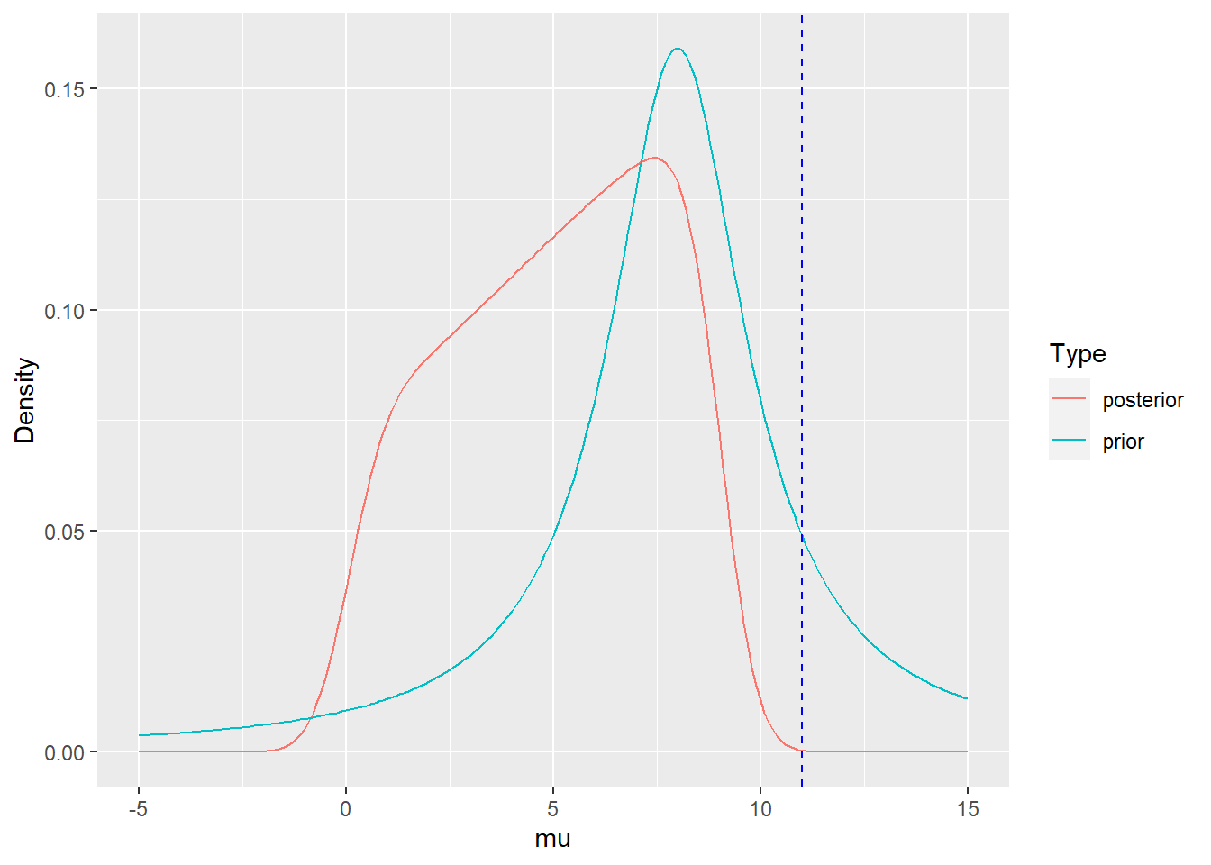
Posterior predictive distribution
Continuous (normal) endpoint
In a pilot study with \(n_1=30\) observations \(x_1,\ldots,x_{n_1}\) a mean \(\bar{x_1}=10.3\) and a standard deviation \(s^2_1=3.8\) were observed.
The function dPred provides the density of the predictive distributions for the observed mean \(\bar{x_2}\) of \(n_2=45\) new observations, using a noniformative prior.
A success criterion is given by: \(\bar{x_2} \ge x_{crit}\), with \(x_{crit}=9.5\).
Then, the probabilty of success is given by the integral over the predictive distribution: \[\int_{-\infty}^{crit} p(\overline{x}_2|\overline{x}_1,s^2_1)dx\] This interval can be calculated by means of the function evalPred.
### Old observations:
m1  <- 10.3
SD  <- 3.8
n1  <- 30

### Posterior predictive distribution for the mean of 20 new observations
Nnew  <- 45
crit  <- 9.5

mx       <- seq(5,15,0.1)
predDist <- dPred(mx,m1=m1,sd1=SD,n1=n1,n2=Nnew,VarKnown=TRUE)
Dist     <- data.frame(mx,predDist)

## probability of succes

pSucc   <- evalPred(m1=m1,sd1=SD,n1=n1,n2=Nnew,crit=crit,VarKnown=TRUE)


Dist2  <- Dist %>% filter(mx >= crit)

PlotPred <- ggplot(Dist,aes(x=mx,y=predDist)) + geom_line(col="blue") +
                   xlab(paste("Observed mean of",Nnew,"new observations")) +                                                 ylab("Posterior predictive density")+
                   geom_vline(xintercept=crit,linetype="dashed",col="red") +
                   geom_area(data=Dist2,aes(x=mx,y=predDist),fill="red",inherit.aes = FALSE,alpha=0.3)+
                   annotate("text",x=9.8,y=0.05,label = paste("P(success)=",round(pSucc,3)),
                            hjust=0,col="red")
print(PlotPred)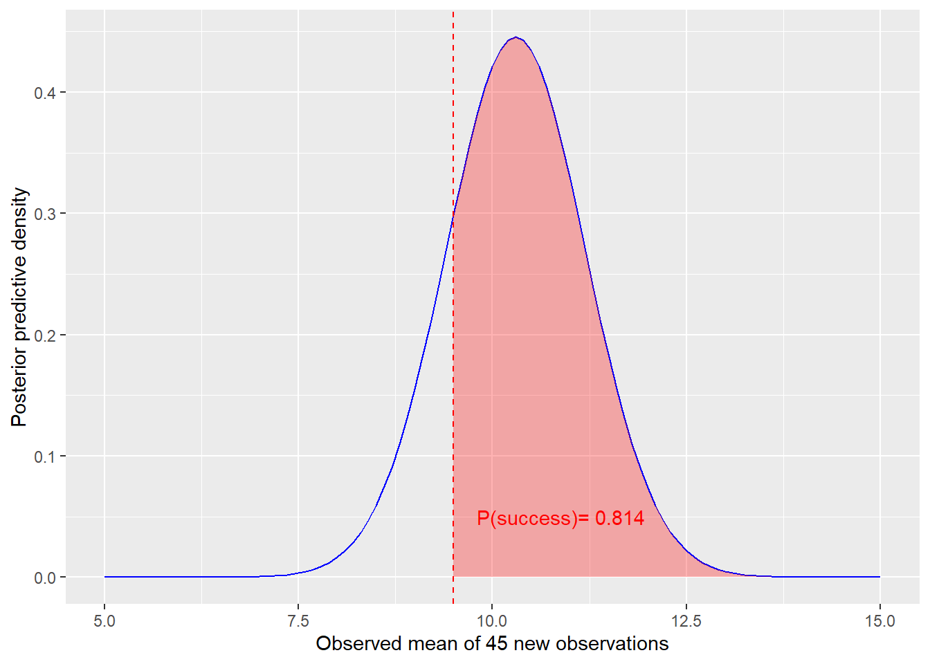
cat("\n prob. Success: ",round(pSucc,3),"\n")
prob. Success: 0.814 Note: Using the function PredDist,an arbitrary prior for the mean can be chosen. However, it much slower tdue to iterated numeric integrations.
Binary endpoint (conjugate analysis)
The posterior predictive distribution for the binomial model with a Beta-prior \(\mathbf{Beta}(\alpha,\beta)\) on the parameter \(\theta\) is the beta-binomial distribution \(\text{Beta-bin} (k,n,\alpha,\beta)\) implemented int the function BetaBinom.
Example:
- Prior on mortality rate: \(\mathbf{Beta} (\alpha=3,\beta=27)\).
- Suppose we now operate on \(n = 10\) patients and observe \(k = 0\) deaths.
- What is the probability that:
- The next patient will survive the operation?: \(\text{Beta-bin} (0,1,\alpha=3+0,\beta=27+10)\)
- That there are 2 or more deaths in the next 20 operations? \(1- \sum_{i=2}^{20}\text{Beta-bin}(i,20,\alpha=3+0,\beta=27+10)\)
## Probability that the next patient will survive the operation
dbetabin(0,10,a=3+0,b=27+10)
[1] 0.4960378## Probability that here are 2 or more deaths in the next 20 operations
1-pbetabin(1,20,a=3+0,b=27+10)[1] 0.4176755## Compare
1-(dbetabin(0,20,a=3+0,b=27+10)+dbetabin(1,20,a=3+0,b=27+10))[1] 0.4176755Finding parameters for the priors in the full normal model with searchPriorVar
A convenient conjugate prior for the full normal model (\(\mu\) and \(\sigma^2\) unknown), is given by (Gelman et al. 1995): \[ \mu|\sigma^2 \sim \mathcal{N}(\mu_0,\sigma^2/\kappa_0)\] \[ \sigma^2 \sim \text{Inv}\!-\!\chi^2(\nu_0,\sigma_0^2).\] Here, $ ^2 ^2(_0,_0^2)$ denotes the scaled inverse-\(\chi^2\) density as implemented in dScaledIChisq and pScaledIChisq (see Gamma_Related_Densities). The function searchPriorVar helps finding parameters for the prior of the variance in the full normal model (scaled inverse-chisq distribution).
First, one has to choose an interval reflecting the prior belief on \(\sigma^2\), i.e. an interval that contains the variance with a predefined coverage probability;
Example:
With 90% probability, the variance is between 9 and 49: \[Prob(9 \le sigma^2 \le 49) = 0.9\]
parm <- searchPriorVar(9,49,0.9)
parm
df scale
8.357316 17.246252 ## Checking the result
x <- rScaledIChisq(100000,parm[1],parm[2]) ## Random numbers
quantile(x,c(0.05,0.95)) 5% 95%
8.972522 48.955196 The degrees of freedom df corresponds to \(\nu_0\) and scale to \(\sigma_0^2\).
Sampling from the Sufficient Statistics of a Normal Distribution
For simulations it is far more efficient to sample directly the sufficient statistics for a given distribution. In the case of the normal model \[x \sim \mathcal{N}(\mu,\sigma^2)\] it is the sample mean and the sample variance \((\overline{x},s^2)\).
The sample mean is distributed as: \[\overline{x} \sim \mathcal{N}(\mu,\frac{\sigma^2}{n})\] where \(n\) denotes the sample size, and the ample variance:
\[s^2 \sim \chi^2_{n-1}\times \frac{\sigma^2}{n-1}\]
The parametrization was chosen in order to be consistent with Bayesian applications (Gelman et al. 1995).
Moments: \(\text{E}(X)=scale; \quad \text{Var}(X)=2\times scale^2/df\).
With this notation, one gets:
\[s^2 \sim \text{Scaled}\!-\!\chi^2(df=n-1,scale=\sigma^2).\] \(\text{Scaled}\!-\!\chi^2(\nu_0,\sigma_0^2)\) scaled inverse-\(\chi^2\) density as implemented in Gamma_Related_Densities.
mu     <- 0
sigma  <- 2
N      <- 5

Nsim    <- 100000 ## Number of simulations


xVar    <- rchisq(Nsim,N-1)/(N-1)*sigma^2

hist(xVar,prob=TRUE,nclas=50,xlab="Sampled variance",main="")
curve(dchisq((N-1)*x/sigma^2,N-1)*(N-1)/sigma^2,ad=TRUE,col=3,lwd=3)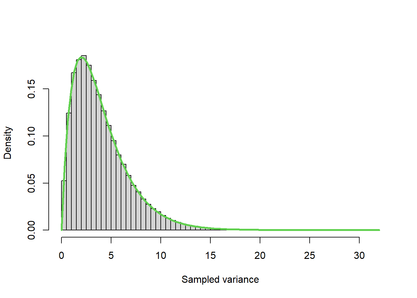
Theoretical background
Probability of Success after Interim Analysis
Mean at IA known
The probability of success (or DDCP) is defined as the probability that the mean of a random variable is greater than a critical value \(x_{crit}\), given the result of an interim analysis \((\sigma^2|\overline{x}_{ia};s_{ia}^2)\). It can be formally written as: \[\begin{equation} \label{PoS} \text{prob}(\overline{x}_{fin} \geq x_{crit}) = \int(1-\Phi(x_{crit}; \theta = \theta_c, \sigma^2 = \sigma_c^2)) \times p(\theta,\sigma^2|\overline{x}_{ia};s_{ia}^2)d\theta d\sigma^2 \quad (1) \end{equation}\]
In \((1)\), \(\Phi\) denotes the normal CDF and \(\theta_c\), \(\sigma_c^2\) (which depend on \(\theta\) and \(\sigma^2\)) are as defined in “Conditional Normal Distributions at an Interim Analysis”.
\(p(\theta,\sigma^2|\overline{x}_{ia};s_{ia}^2)\) is the posterior density of the parameters \(\theta\) and \(\sigma^2\), given \((\overline{x}_{ia};s_{ia}^2)\).
Interval for mean known at IA
If at the interim analysis only an interval for the mean is known \[\theta_0 \leq \overline{x}_{ia} \leq \theta_1,\] the conditional probability for \(\overline{x}_{fin}\) is given as
\[\begin{equation} \text{Prob}(\overline{x}_{fin} \geq x_{crit}| \overline{x}_{ia} \in [\theta_0,\theta_1], \theta, \sigma^2) = \frac{p(\overline{x}_{fin} \geq x_{crit}, \overline{x}_{ia} \in [\theta_0,\theta_1]|\theta,\sigma^2 )}{p(\overline{x}_{ia} \in [\theta_0,\theta_1]| \theta, \sigma^2)} \quad(2) \end{equation}\]
The joint distribution of \((\overline{x}_{ia},\overline{x}_{fin})\) is given in “Conditional Normal Distributions at an Interim Analysis”.
In order to obtain the PoS, \((2)\) has again to be integrated over the posterior distribution of the parameters as in \((1)\).
Multivariate normal mean
The multivariate case is analogous and can be easily derived; here we omit it for simplicity.
Relation to conditional and predictive power
The variance \(\sigma^2\) is often assumed to be known and the integration in\((1)\) is carried out over a posterior density for \(\theta\) alone. For \(\sigma^2\), \(s_{ia}^2\) is imputed.
With known \(\sigma^2\), the \(1-\alpha\) quantile of \(\mathcal{N}(\theta, \sigma^2)\) can be be chosen as \(x_{crit}\). In this case \((1)\) becomes the predictive power. If the values such as used for a ‘classical’ power calculation are chosen for \(\theta\) and \(\sigma^2\) in \(x_{crit}, (1)\) reduces to: \[\begin{equation} \label{CondPow1} \text{prob}(\overline{x}_{fin} \geq x_{crit}) = 1-\Phi(x_{crit}; \theta = \theta_c, \sigma^2 = \sigma_c^2) \end{equation}\]
Conditional Normal Distributions at an Interim Analysis
Let \(x \sim \mathcal{N}(\theta, \sigma^2)\) and \(\overline{x}_{ia}=\hat{\theta}_{ia}\) be the (observed) mean of \(n_{ia}\) observations at the time point of the interim analysis (IA) and \(s^2_{ia}\) the corresponding sample variance. Then the conditional density of the observed mean \(\overline{x}_{fin}\) at the final analysis with \(n_{fin}\) observations is given by: \[\overline{x}_{fin}|\overline{x}_{ia} \sim \mathcal{N}(\theta_c, \sigma_c^2)\] where
\[\theta_c=\frac{n_{ia}}{n_{fin}}\overline{x}_{ia}+(1-\frac{n_{ia}}{n_{fin}})\theta\] and
\[\sigma_c^2=\frac{\sigma^2}{n_{fin}} (1 - \frac{n_{ia}}{n_{fin}})\]
Multivariate case
The multivariate case is analogous; the conditional distribution of the observed multivariate mean \(\overline{\mathbf{x}}_{fin}\) given \(\overline{\mathbf{x}}_{ia}\) and the observed covariance matrix \(\Sigma_{ia}\) is:
\[ \overline{\mathbf{x}}_{fin}|\overline{\mathbf{x}}_{ia} \sim \mathcal{N}(\mathbf{\theta}_c, \Sigma_c)\]
where \[\mathbf{\theta}_c=\frac{n_{ia}}{n_{fin}} \overline{\mathbf{x}}_{ia}+(1-\frac{n_{ia}}{n_{fin}})\mathbf{\theta}\] and \[\Sigma_c=\frac{\Sigma}{n_{fin}} (1 - \frac{n_{ia}}{n_{fin}})\]
Outline of proof (univariate case)
In a case of \(k=1\ldots n_{fin}\) analyses (\(n_{fin}-1\) interim analyses), the estimator
\[\mathbf{\hat{\theta}}=(\mathbf{\bar{x}}_1, \ldots,\mathbf{\bar{x}}_n)\]
is (multivariate) normally distributed with expected value \((\theta,\ldots,\theta)\) and covariance matrix: \[\begin{equation} \label{distIA} \sigma^2 \times \begin{pmatrix} n_1^{-1} & n_2^{-1} & n_3^{-1} & \cdots & n_{fin}^{-1}\\ n_2^{-1} & n_2^{-1} & n_3^{-1} & \cdots & n_{fin}^{-1}\\ n_3^{-1} & n_3^{-1} & n_3^{-1} & \cdots & \vdots\\ \vdots &\vdots & & \ddots & \vdots\\ n_{fin}^{-1} & n_{fin}^{-1} & \ldots & \ldots & n_{fin}^{-1}\\ \end{pmatrix} \end{equation}\]
The well-known theorem on conditional normal distributions, where \(\mathbf{x}\) is partitioned as follows \[\mathbf{x} = \begin{bmatrix} \mathbf{x_1}\\ \mathbf{x_2} \end{bmatrix}, \mathbf{\theta}= \begin{bmatrix} \mathbf{\theta_1}\\ \mathbf{\theta_2} \end{bmatrix}\] \[\mathbf{\Sigma}= \begin{bmatrix} \mathbf{\Sigma_{11}} & \mathbf{\Sigma_{12}}\\ \mathbf{\Sigma_{12}} & \mathbf{\Sigma_{22}}\\ \end{bmatrix}\]
states that the distribution of \(\mathbf{x_2}\) conditional on \(\mathbf{x_1}=\mathbf{\hat{\theta_1}}\) is multivariate normal with expected value \[\mathbf{\theta_2}+\mathbf{\Sigma}_{12}\mathbf{\Sigma}_{11}^{-1} \times (\mathbf{x_1} - \mathbf{\theta_1})\] and covariance matrix \[\mathbf{\Sigma}_{22} - \mathbf{\Sigma}_{12}\mathbf{\Sigma}_{11}^{-1}\mathbf{\Sigma}_{12}\]
From that, the result follows immediately.
Conjugate Bayesian Estimation of the Full Normal Model
Noninformative Prior
Be \({x_1,x_2, \dots, x_n}\) i.i.d. with \(x_i \sim \mathcal{N}(\mu,\sigma^2)\) with unknown \(\mu\) and \(\sigma^2\). Denoting
\[ s^2=\frac{1}{n-1}\sum_{i=1}^{n}(x-\bar{x})^2\] and \[\bar{x} = \frac{1}{n}\sum_{i=1}^n x_i\] the posterior density (noninformative prior) for \(\sigma^2\) is: \[ \sigma^2|\{x_i\} \sim \text{Scaled-inv}\!-\!\chi^2(n-1,s^2).\] The posterior density for the precision \(\tau\) is: \[ \tau|\{x_i\} \sim \text{Scaled}\!-\!\chi^2(n-1,s^{-2})\] and the posterior for \(\mu\) is: \[\mu|\{x_i\} \sim \text{t}_{n-1}(\bar{x},s^2/n),\] where \(\text{t}_{\nu}(\mu,\sigma^2)\) is the Student-t distribution with \(\nu\) degrees of freedom, location \(\mu\) and scale \(\sigma\).
Conjugate prior for variance
A convenient conjugate prior for the full normal model (\(\mu\) and \(\sigma^2\) unknown), is given by: \[ \mu|\sigma^2 \sim \mathcal{N}(\mu_0,\sigma^2/\kappa_0)\] \[ \sigma^2 \sim \text{Inv}\!-\!\chi^2(\nu_0,\sigma_0^2).\]
Marginal posterior distributions
Posterior distribution for \(\sigma^2\)
\[\sigma^2|\{x_i\} \sim \text{Scaled-inv}\!-\!\chi^2(\nu_n,\sigma^2_n),\]
where:
\[\nu_n = \nu_0 + n\]
\[\sigma^2_n = \frac{1}{\nu_n} \left[\nu_0\sigma_0^2+(n-1)s^2+\frac{\kappa_0 n}{\kappa_0+n}(\mu_0-\bar{x})^2 \right].\]
Posterior distribution for \(\mu\)
\[\mu|\{x_i\} \sim \text{t}_{\nu_n}(\mu_n,\sigma_n^2/\kappa_n),\] with \[\kappa_n = \kappa_0 +n\] and \[\mu_n = \frac{\kappa_0}{\kappa_0 + n} \mu_0 + \frac{n}{\kappa_0 + n}\bar{x}.\]
Posterior predictive distribution (noninformative prior)
The mean \(\bar{x}_{new}\) of new (independent) future observations \(x_{n+1}, \ldots,x_{n+m}\) having observed \(\{\bar{x}_{old}.s^2_{old}\}\), the mean and variance of \(x_1,\ldots,x_n\) is distributed as: \[\bar{x}_{new}|\bar{x}_{old},s^2_{old} \sim t_{n-1} \left( \bar{x}_{old},s^2_{old}(\frac{1}{n}+\frac{1}{m})\right)\]
The Beta-Binomial distribution
The Beta distribution is a conjugate distribution of the binomial distribution. This fact leads to an analytically tractable compound distribution where one can think of the parameter p in the binomial distribution as being randomly drawn from a beta distribution. Namely, if \[X \sim \text{Bin}(n,\pi)\] \[Prob(X=k|n,\pi)=\binom{n}{k}\pi^k(1-\pi)^{n-k}\] where \(\text{Bin}(n,\pi)\) stands for the binomial distribution, and where \(\pi\) is a random variable with a Beta distribution. \[p(\pi|\alpha,\beta) = \text{Beta}(\pi|\alpha,\beta)=\frac{\pi^{\alpha-1}(1-\pi)^{\beta-1}}{\text{Beta}(\alpha,\beta)}\] then the compound distribution is given by \[f(k|n,\alpha,\beta)=\int_0^1 P(k|s,n)\times p(s|\alpha,\beta)ds\]
\[=\binom{n}{k} \int_0^1 s^{k+\alpha-1} \times (1-s)^{n-k+\beta-1}ds=\binom{n}{k} \frac{\text{B}(k+\alpha,n-k+\beta)}{\text{B}(\alpha,\beta)}\]
\(\Gamma\) Distribution
Parametrizations
A \(\Gamma(\alpha,\beta)\) density has the PDF: \[f(x)=\frac{1}{\Gamma(\alpha)\beta^{\alpha}}x^{\alpha -1}e^{-x/\beta}\] for \(x > 0\). The parameter \(\alpha\) is called and \(\beta\) . Often, it is parameterized with the -parameter \(\lambda=1/\beta\)
Properties
Moments: \(\text{E}(X)=\alpha\beta=\alpha/\lambda; \quad \text{Var}(X)=\alpha\beta^2=\alpha/\lambda^2; \quad \text{Skewness}=2/\sqrt{\alpha}\).
If \(X_i \sim \Gamma(\alpha_i,\beta)\quad \text{then}\quad \sum_i X_i \sim \Gamma(\sum_i \alpha_i,\beta)\)
Be \(c >0\), then \(cX \sim \Gamma(\alpha,c\beta)\).
\(\text{Inv}\!-\!\Gamma\) Distribution
If \(X \sim \Gamma(\alpha,\beta)\), then \(Y=1/X \sim \text{Inv}\!-\!\Gamma(\alpha,scale=1/\beta)\).
Properties
PDF: \(f(x)=\frac{\beta^{\alpha}}{\Gamma(\alpha)}x^{-\alpha -1}e^{-\beta/x} \quad(x>0)\)
Moments: \(\text{E}(X)=\frac{\beta}{\alpha-1} \quad(\alpha>1); \quad \text{Var}(X)=\frac{\beta^2}{(\alpha-1)^2(\alpha-2)} \quad(\alpha>2)\).
\(\text{Scaled}\!-\!\chi^2\) distribution
If \(X \sim \chi^2(df)\) then \(cX \sim \text{Scaled}\!-\!\chi^2(df,scale=df\times c)\).
The parametrization was chosen in order to be consistent with Bayesian applications .
Moments: \(\text{E}(X)=scale; \quad \text{Var}(X)=2\times scale^2/df\).
\(\text{Scaled-inv}\!-\!\chi^2\) distribution
If \(X \sim \text{Scaled}\!-\!\chi^2(df,scale=df\times c)\) then \(1/X \sim \text{Scaled-inv}\!-\!\chi^2(df,scale=1/(df\times c))\).
Moments: \(\text{E}(X)=\frac{df\times scale}{df-2} \quad (df>2); \quad \text{Var}(X)=\frac{2df^2\times scale^2}{(df-2)^2(df-4)} \quad (df > 4)\).
Relation between Distributions
| \(\chi^2(df=\nu)\) | \(\Gamma(\alpha=\frac{\nu}{2},\beta=2\)) |
| \(\text{Scaled}\!-\!\chi^2(df=\nu,scale=s^2)\) | \(\Gamma(\alpha=\frac{\nu}{2},\beta=\frac{2s^2}{\nu})\) |
| \(\text{Scaled-inv}\!-\!\chi^2(df=\nu,scale=s^2)\) | \(\text{Inv}\!-\!\Gamma(\alpha=\frac{\nu}{2}, scale=\frac{\nu s^2}{2})\) |
References
Dmitrienko, Alexei, and Ming-Dauh Wang. 2006. “Bayesian Predictive Approach to Interim Monitoring in Clinical Trials.” Stat. Med. 25 (13): 2178–95.
Gelman, A., J. B. Carlin, H. S. Stern, and D. B. Rubin. 1995. Bayesian Data Analysis. Chapman & Hall.
Proschan, M., K. Lan, and J. Wittes. 2006. Statistical Monitoring of Clinical Trials: A Unified Approach. Springer, New York.