# Load necessary packages
library(bpp)
library(rpact)Probability of success of a clinical trial: choice of the prior
Setup
About this document
This short note discusses aspects for the choice of the prior when computing DDCP. More specifically, it describes how we can specify the pessimistic prior that had been introduced in Rufibach et al. (2016) and used in the MIRROS case study.
The tutorial on strategic context offers further points to consider when deriving a prior.

Prior choice
Given that typically, estimates of parameters we are building our priors for, e.g. mean differences or log hazard ratios, can be well approximated by a Normal distribution the latter is often our first choice for a prior distribution family. Note that the Normal prior might actually carry quite a bit of information, even and often especially so when it is based on few events. Then, the variance is large implying that the prior assigns large weights to potentially completely implausible values for the effect of interest. This aspect is discussed in Rufibach et al. (2016).
However, depending on the scientific context, other priors might also be sensible, e.g. if you want to be more agnostic on your underlying effect. An example is provided in the MIRROS case study.
What information can / should be used to define the prior?
Ideally, prior information comes from evidence outside of the trial you are planning, i.e. the prior should not be influenced by the effect size that is assumed for the trial DDCP is intended to compute. However, as the effect size you assume to compute power for the trial of interest is by itself already a reflection of the synthesis of available evidence, often this cannot be separated so clearly.
But the recommendation is still to inform the prior separately from the assumptions about the trial of interest, as much as possible.
Specification of the pessimistic prior
Next, as an alternative to a Normal prior, we will discuss how to specify the “pessimistic prior” initially introduced in Rufibach et al. (2016) .
In the function dUniformNormalTails that is available in the package bpp the pessimistic density is parametrized as follows:
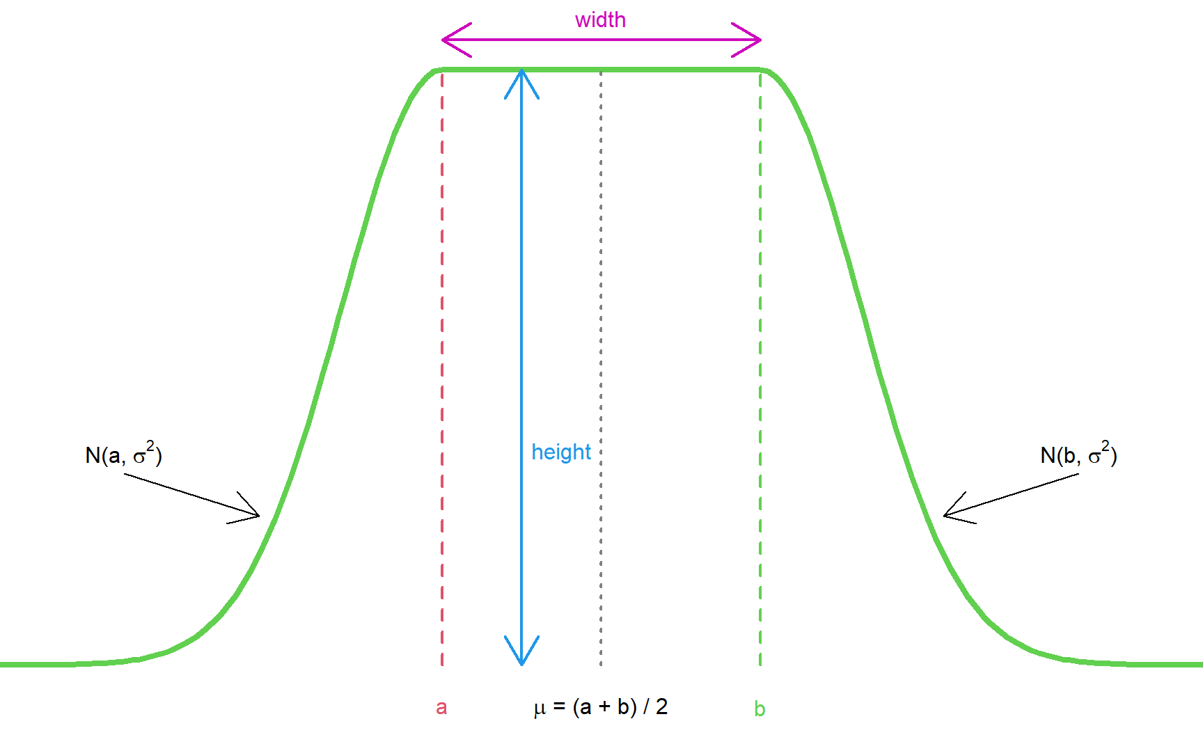
We need to specify the following parameters:
- The width of the horizontal stretch. In terms of determining that it is typically easiest to define it through the endpoints \(a\) and \(b\) of the horizontal stretch, respectively. \(a\) and \(b\) define the interval on which you want to be rather agnostic about the effect size of interest.
- The center \(\mu\) of the prior (corresponding to its mean) which again can be computed from \(a\) and \(b\) as \(\mu = (a + b) / 2\).
- Finally,
dUniformNormalTailsrequires specification of the height of the horizontal stretch. Together with the constraint that the density integrates to 1 this also implicitly defines the variance \(\sigma^2\) of the two Normal tails. The height can be freely chosen under the constraint that there is enough area “left” for the tails, i.e. height \(\cdot\) width must be strictly below 1. One way to get rid of this degree of freedom is to require a certain probability for the prior to be above or below a threshold of interest, see below in the Section “How pessimistic is the pessimistic prior?”.
Note that the parametrization in the function dUniformNormalTails in the package bpp that is depicted above is slightly different from the one in Rufibach et al. (2016): the latter parametrizes \(\sigma^2\) and the height follows from the area constraint.
Example for a continuous endpoint
Now let us illustrate construction of a prior for a continuous endpoint. To this end we borrow from this example from adaptr. The pivotal trial is planned as follows:
# Example of a standard trial:
# - targeted mean difference is 10 (alternative = 10)
# - standard deviation in both arms is assumed to be 24 (stDev = 24)
# - two-sided test (sided = 2), type I error 0.05 (alpha = 0.05) and power 80% (beta = 0.2)
d <- 10
s <- 24
sampleSize <- getSampleSizeMeans(alternative = d, stDev = s, sided = 2,
                                 alpha = 0.05, beta = 0.2)
mdd <- sampleSize$criticalValuesEffectScaleUpper[1, 1]
mdd
[1] 7.00557So the MDD for this trial is approximately 7.
Now assume we have run a randomized Phase 2 (or can inform the prior based on external data) that shows the following results:
# randomized Phase 2 trial:

# observed mean difference
mu2 <- 13.1

# observed standard error
sig2 <- 34.2
One option would be to specify a Normal prior based on these results, with mean \(13.1\) (or a shrunken version of that) and variance \(34.2^2\). This is the red line in the figure below. However, here we want to be more agnostic (or pessimistic) as follows:
par(las = 1, mar = c(4.5, 4.5, 2, 1), mfrow = c(1, 1))
plot(0, 0, type = "n", xlim = c(-100, 125), ylim = c(0, 0.0125),
     xlab = "mean difference", ylab = "density", main = "")
title("Pessimistic prior density q for mean difference", line = 0.7)
legend("topleft", c("normal prior", "pessimistic prior"), lty = 1, col = 2:3, lwd = 3, bty = "n")

# normal prior based on Phase 2 trial
x <- seq(mu2 - 200, mu2 + 200, by = 0.1)
lines(x, dnorm(x, mean = mu2, sd = sig2), col = 2, lwd = 3)

# now determine pessimistic prior
# flat stretch and slight shift to left
w2 <- 50   # half of width of horizontal stretch
shift <- 10
a <- (mu2 - shift) - w2
b <- (mu2 - shift) + w2
width <- (b - a)
height <- 0.006
mu <- (a + b) / 2

# plot the pessimistic prior
lines(x, dUniformNormalTails(x, mu = mu, width = width, height = height),
      lwd = 2, col = 3)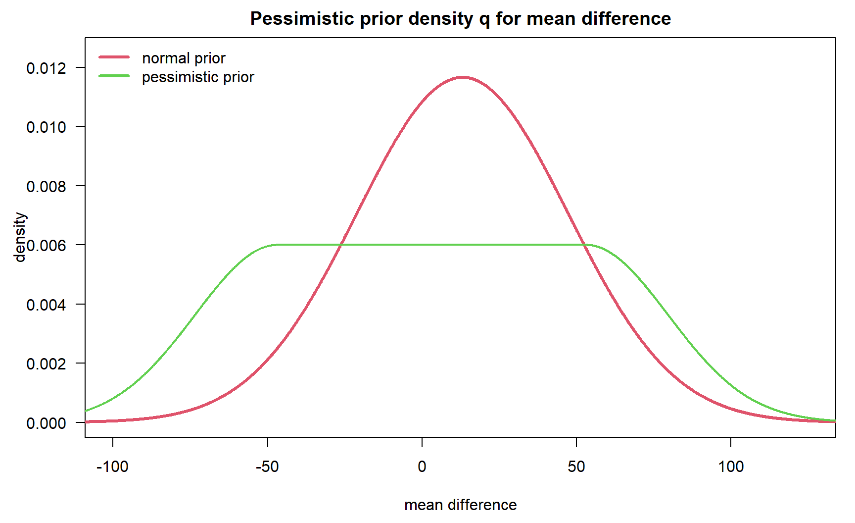
So we do not favor any effect between -46.9 and 53.1. This prior can now be used to compute DDCP as follows:
# standard error of effect estimate at final analysis
finalSE <- sqrt(s ^ 2 + s ^ 2)

# DDCP at TPP
p_tpp <- bpp(prior = "flat", successmean = d, finalSE = finalSE,
             priormean = mu, width = width, height = height)

# DDCP at MDD
p_mdd <- bpp(prior = "flat", successmean = mdd, finalSE = finalSE,
             priormean = mu, width = width, height = height)

# note that the function bpp() is defined such that effects smaller
# than successmean are "successes"
1 - c(p_tpp, p_mdd)
[1] 0.4597229 0.4771882How pessimistic is the pessimistic compared to a Normal prior?
No general statement can be made. However, the wider the flat part the more agnostic the prior is about the underlying effect size. To illustrate and compare the two priors computation of probabilities to be above or below certain effect sizes of interest might be informative:
# Normal prior probabilities to be below 0 or above 20:
lims <- c(0, 20)
pnorm1 <- pnorm(lims[1], mean = mu2, sd = sig2)
pnorm2 <- 1 - pnorm(lims[2], mean = mu2, sd = sig2)
c(pnorm1, pnorm2)
[1] 0.3508447 0.4200544Compare this to the probabilities for the pessimistic prior:
# pessimistic prior probabilities to be below 0 or above 20:
flat1 <- pUniformNormalTails(x = lims[1], mu = mu, width = width, height = height)
flat2 <- 1 - pUniformNormalTails(x = lims[2], mu = mu, width = width,
                                 height = height)
c(flat1, flat2)
[1] 0.4813997 0.3985991So indeed, probabilities for the pessimistic prior to be below 0 are higher and to be above 20 lower than for the Normal prior. We can also compare the DDCP values directly:
# DDCP at TPP
p2_tpp <- bpp(prior = "normal", successmean = d, finalSE = finalSE,
              priormean = mu2, priorsigma = sig2)

# DDCP at MDD
p2_mdd <- bpp(prior = "normal", successmean = mdd, finalSE = finalSE,
             priormean = mu2, priorsigma = sig2)

1 - c(p2_tpp, p2_mdd)
[1] 0.5256493 0.5503256So here indeed, DDCP values for the Normal prior are higher compared to the pessimistic prior, so more “optimistic”.
Example for a time-to-event endpoint
Specification of a pessimistic prior for a time-to-event endpoint is discussed in detail in the MIRROS case study.
References
Rufibach, K., H. U. Burger, and M. Abt. 2016. “Bayesian Predictive Power: Choice of Prior and Some Recommendations for Its Use as Probability of Success in Drug Development.” Pharm. Stat. 15: 438–46.
Rufibach, K., P. Jordan, and M. Abt. 2016. “Sequentially updating the likelihood of success of a Phase 3 pivotal time-to-event trial based on interim analyses or external information.” J Biopharm Stat 26 (2): 191–201. http://dx.doi.org/10.1080/10543406.2014.972508.