Probability of success of a clinical trial: backengineer a prior from a generic PTS

Author

Affiliation

Kaspar Rufibach

Methodology, Collaboration, and Outreach Group, PD DSS, Roche Basel

Setup

# Load necessary packages
library(bpp)
library(rpact)

About this document

Ideally, to compute DDCP one proceeds as follows:

1. Collect prior evidence about the treatment effect of interest.
2. Construct a prior distribution based on that evidence, as discussed here. As discussed here determining a prior is a task that involves the entire trial team, not “only” the statistician.
3. Develop the design of the trial you want to compute DDCP for.
4. Compute DDCP as discussed here.
5. Keep an eye on the strategic context.

Sometimes, teams prefer to use a generic PTS for their, say, Phase 3 trial. This implies that you omit Steps 1.-2. and 4. above. However, at times, it may be useful to know which prior could have led to the computation of a DDCP value corresponding to the chosen generic PTS. For example:

• You need a prior to illustrate to the team what implicit assumptions on prior evidence they are actually making with the chosen generic PTS. If the back-engineered prior looks too optimistic or pessimistic compared to the known evidence, do not use the generic PTS. Modify the prior distribution and calculate the DDCP.
• You want to potentially compute an updated DDCP value to replace the generic PTS, because you have acquired new evidence, e.g.
  • trial-external evidence,
  • an interim analysis of your trial.

See here for details.

In this tutorial we describe how to “back-engineer” a Normal and pessimistic prior, starting from the generic PTS chosen value and Phase 3 study design, share corresponding code, and point to Roche projects where these methods have been used.

Note that the general recommendation is that teams should really try to come up with quantifying prior evidence, derive a prior from that and compute DDCP, instead of using a generic PTS.

Examples from projects

Priors have been back-engineered in projects before. Below are the links to the successR tutorials where this is documented:

• Back-engineering of a Normal prior in Gazyva program. Purpose: allow for updates from external evidence and interim analyses.
• Back-engineering of a Normal prior in JACOB trial. Purpose: allow for updates from interim analysis.
• Back-engineering of a pessimistic prior in MIRROS trial. Purpose: explore how much a futility interim changes PTS and use that to tune the futility interim boundary.

Back-engineer a Normal prior

Assume that the team has the following task:

• A generic PTS of a Phase 3 trial of 65% has been adopted.
• What Normal prior does this correspond to?

The first observation is that we have one degree of freedom “too much”: We must choose the mean \(\delta_0\) and the standard deviation \(\sigma_0\) of our Normal prior. It appears sensible to

• select the standard deviation a priori to quantify how much “evidence” our prior information should correspond to,
• and then tune the prior mean to match the above initial generic PTS.

In order to determine, for a given \(\sigma_0\), the mean of a Normal prior \(\delta_0\) that gives a DDCP of 65%, we can invert the well-known formula for DDCP assuming a Normal prior and normally distributed endpoint of the Phase 3 trial, see the methodology tutorial. Simple manipulation of that equality gives

\[ \delta_0 \ = \ \delta_\text{suc} - \Phi^{-1}(\text{assurance})\sqrt{\sigma_\text{fin}^2 + \sigma_0^2}. \]

Illustration using a time-to-event endpoint

Design of pivotal trial

First, we specify all the quantities of the pivotal trial for which we want the DDCP to match our generic PTS.

# specifications of exemplary Phase 3 trial with time-to-event endpoint
alpha <- 0.05
beta <- 0.2
hr <- 0.76

design <- getDesignGroupSequential(sided = 2, alpha = alpha, beta = beta,
                                   informationRates = 1,
                                   typeOfDesign = "asOF")
sampleSize <- getSampleSizeSurvival(design = design, hazardRatio = hr)

# number of events
nevents <- ceiling(sampleSize$maxNumberOfEvents)
nevents

[1] 417

# MDD
hrMDD <- sampleSize$criticalValuesEffectScaleLower[1, 1]
hrMDD

[1] 0.8253122

So the assumptions for our pivotal trial are:

• Two-sided significance level of \(\alpha = 0.05\).
• 1(treatment):1(control) randomization.
• 80% power to detect an overall hazard ratio of 0.76 using a standard log-rank test. This requires 417 events.
• No interim analysis.
• The minimal detectable difference amounts to 0.825.

Derivation of prior

In the case of a time-to-event endpoint (and assuming proportional hazards) the standard deviation of the estimate of the log of the hazard ratio depends on the number of events, i.e. in the case of a 1:1 randomized Phase 2 trial we would have \(\sigma_0^2 = 4 / d_0\) with \(d_0\) the number of events in the Phase 2 trial. One can either

• simply pick \(d_0\) or
• consider a few scenarios as follows:

# determine number of events the prior knowledge should be worth of
pts1 <- 0.65
n0 <- c(25, 50, 100, 200)

# assume 1:1 randomization
propA0 <- 0.5   
fac0 <- (propA0 * (1 - propA0)) ^ (-1)
sd0 <- sqrt(fac0 / n0)
  
# standard error of effect estimate at final analysis
propA <- 0.5
fac <- (propA * (1 - propA)) ^ (-1)
finalSE <- sqrt(fac / nevents)

# MDD on log-scale --> success criteria
successmean <- log(hrMDD)

# now find the prior means that correspond to this choice of pts1 and n0
delta0 <- successmean - qnorm(pts1) * sqrt(finalSE ^ 2 + sd0 ^ 2)

# hazard ratios at which priors are centered
round(exp(delta0), 3)

[1] 0.704 0.735 0.757 0.772

The fewer prior events we assume the wider the prior density gets. This implies that the prior mean needs to be further away from the null hazard ratio of 1 to still give an initial DDCP of 65%. The priors look as follows:

xli <- log(c(0.35, 1.6))
yli <- c(-0.1, 2.9)
par(las = 1, mar = c(9, 5, 2, 1), mfrow = c(1, 1))
plot(0, 0, type = "n", xlim = xli, ylim = yli, xlab = "", ylab = "density", 
     main = "Normal prior densities")
basicPlot(leg = FALSE, IntEffBoundary = NA, IntFutBoundary = NA, successmean = NA, priormean = NA)
segments(log(hrMDD), 0, log(hrMDD), 3, col = "brown", lwd = 4, lty = 2)
legend(-0.8, 2, "MDD", lwd = 4, lty = 2, bty = "n", col = "brown")

# now add prior densities and corresponding DDCP values
thetas <- seq(0.3, 2.7, by = 0.01)
lthetas <- log(thetas)
for (i in 1:length(n0)){lines(lthetas, dnorm(lthetas, mean = delta0[i], sd = sqrt(fac0 / n0[i])), 
                     col = i + 1, lwd = 4, lty = 1)}
legend("topleft", legend = paste(n0, " / ", round(exp(delta0), 3)), col = 1 + 1:length(n0), 
       lwd = 4, lty = 1, title = "Number of prior events and hazard ratios:", bty = "n")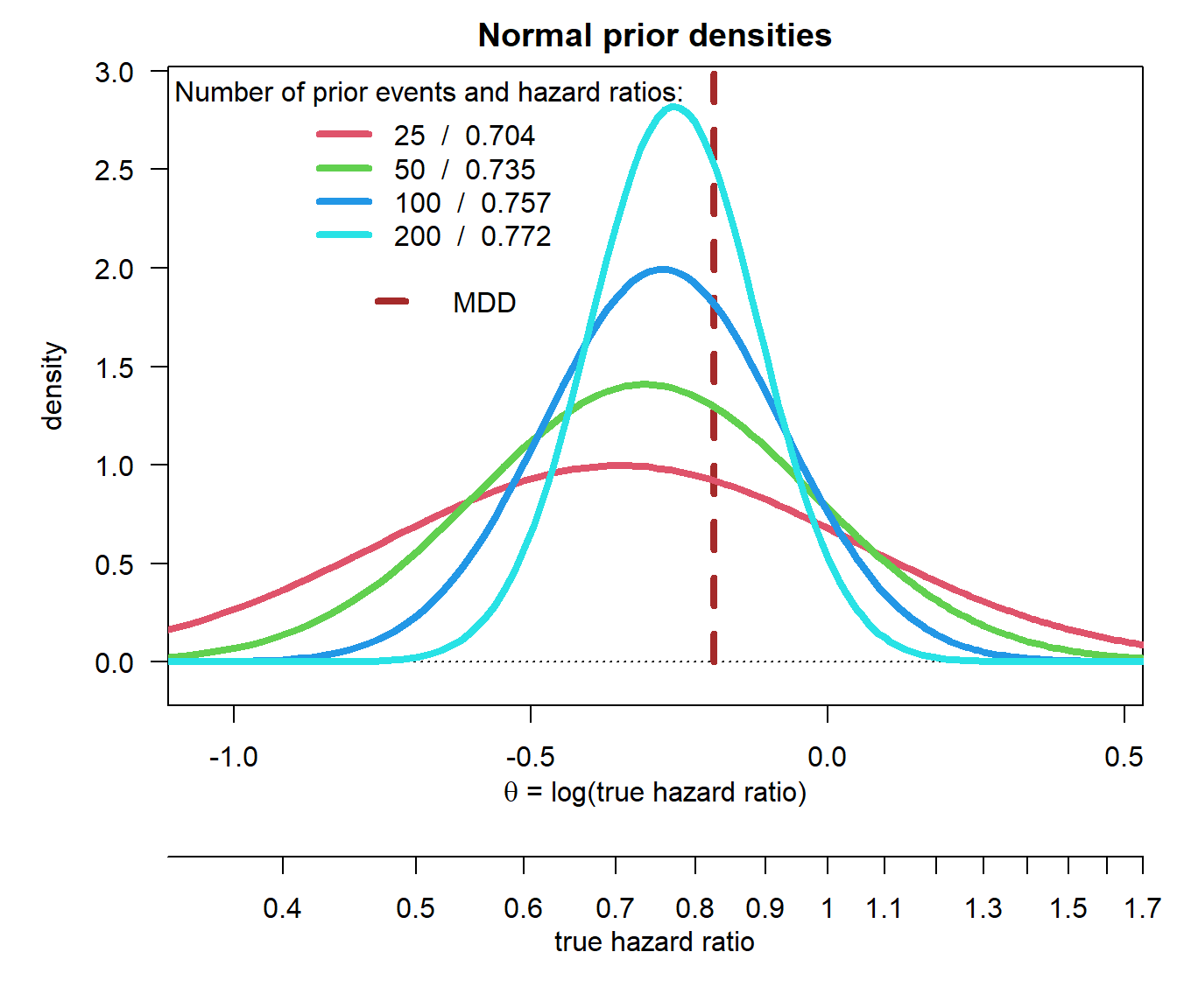

Verification

We can verify the computations:

bpp(prior = "normal", successmean = successmean, finalSE = finalSE, 
    priormean = delta0, priorsigma = sd0)

[1] 0.65 0.65 0.65 0.65

Back-engineer a pessimistic prior

Assume that the team has the following task:

• A generic PTS of a Phase 3 trial of 65% has been adopted.
• What pessimistic prior does this correspond to?

For a pessimistic prior we even have more degrees of freedom: As described in the tutorial on prior choice we need to choose in total four parameters. Below we follow the arguments used in MIRROS to do that. Note further that, as opposed to the Normal prior, there is no closed-form formula we can invert analytically for a parameter of interest.

Illustration using a time-to-event endpoint

Design of pivotal trial

We use the same specifications of the pivotal trial as for the Normal prior example above.

Derivation of prior

To set up DDCP based on a generic PTS, the following considerations were made:

• Given that we want to compute generic PTS for a Phase 3 trial one should be somewhat confident that the probability that the hazard ratio exceeds 1 should be small.
• Similarly, it is considered unlikely that the hazard ratio is below 0.55.
• In order not to favor an HR in this range the pessimistic prior introduced in Rufibach et al. (2016) was chosen, see the tutorial on prior choice.
• Finally, the prior should be tuned such that the DDCP to beat the MDD hazard ratio of 0.83 amounts to \(p_{P3} = 0.65\).

The pessimistic prior is introduced in Rufibach et al. (2016). A discussion why such a prior might be preferred over a Normal prior is provided in the tutorial on choice of prior. The parametrization in the function dUniformNormalTails in the package bpp that is used below is slightly different from the paper. Note that when considering the hazard ratio the prior has to be parametrized on the log-scale. We have four parameters that we need to set:

ea <- 0.55
eb <- 1
a <- log(ea)
b <- log(eb)
width <- b - a
height <- 1.3

priormean <- (a + b) / 2
exp(priormean)

[1] 0.7416198

• The width \(b - a\) of the horizontal stretch. It is easiest to define this through the endpoints \(a = \log(0.55)\) and \(b = \log(1)\), respectively.
• The center of the prior: we set this here at a hazard ratio of \(\exp\Bigl(\frac{\log(0.55) + \log(1)}{2}\Bigr) = \log(0.74)\), i.e. in the middle of \(a\) and \(b\) on log-scale.
• By choosing the height of the horizontal stretch we automatically determine the width of the tails, because the area under the resulting density needs to integrate to 1. We can play around with this height to fine tune our prior - we set this height to \(h = 1.3\).

These choices give the following prior:

par(las = 1, mar = c(8, 6, 2, 1), mfrow = c(1, 1)) 
plot(0, 0, type = "n", xlim = log(c(0.45, 1.23)), ylim = c(-0.1, 2), xlab = "", ylab = "density", 
     main = "") 
title(expression("Pessimistic prior density "*q[0]*" for "*theta), line = 0.7) 
basicPlot(leg = FALSE, IntEffBoundary = NA, IntFutBoundary = NA, successmean = NA, priormean = NA) 
thetas <- seq(0.35, 7.5, by = 0.005)
lthetas <- log(thetas)
lines(lthetas, dUniformNormalTails(lthetas, mu = priormean, width = width, height = height), 
      lwd = 2, col = 3)

segments(log(hrMDD), 0, log(hrMDD), 2, col = "brown", lwd = 4, lty = 2)
legend(-0.6, 2, "MDD", lwd = 4, lty = 2, bty = "n", col = "brown")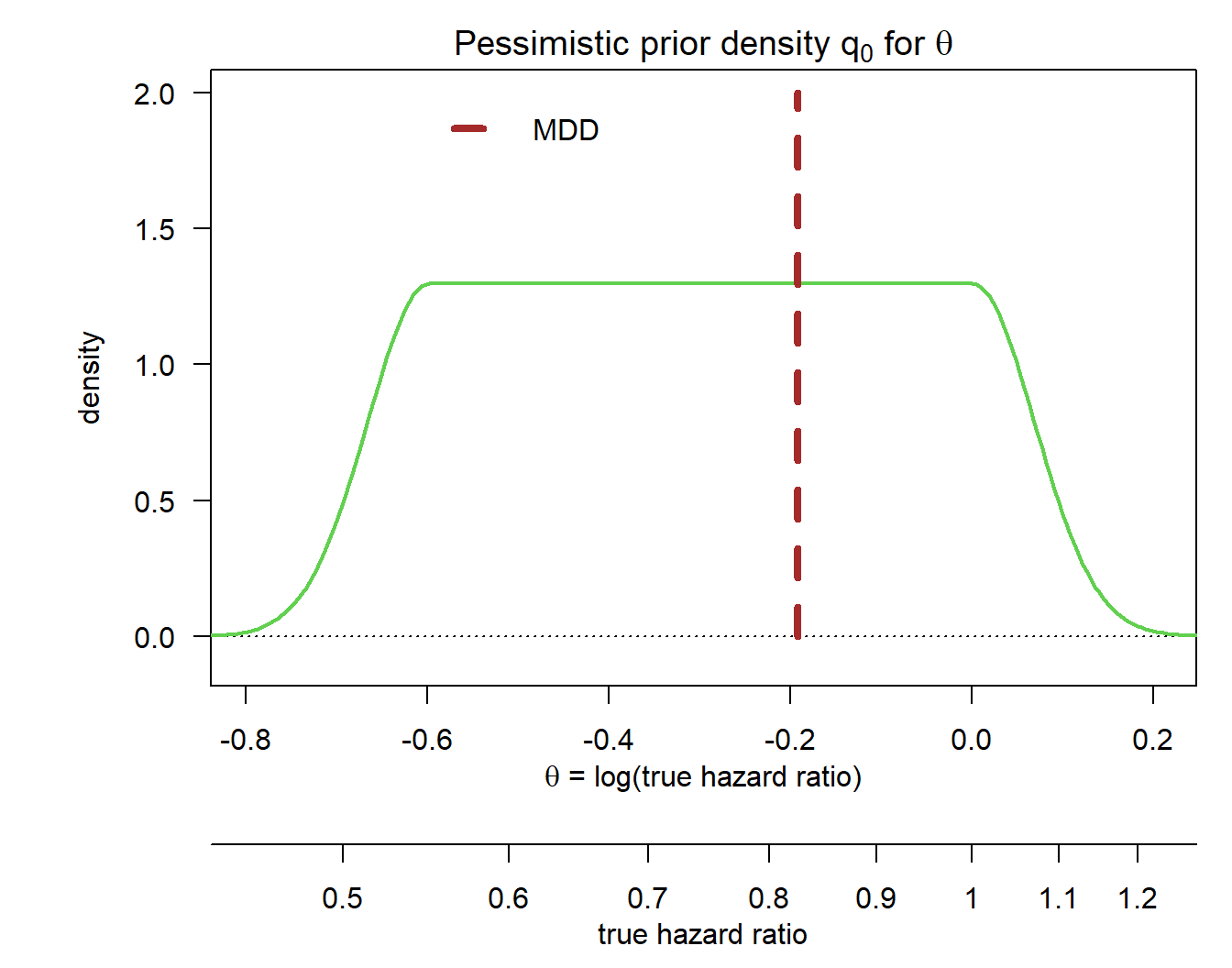

Verification

We can compute probabilities of potential interest based on this prior:

# DDCP at TPP
p_tpp <- bpp_t2e(prior = "flat", successHR = hr, d = nevents, priorHR = exp(priormean), 
                 propA = 0.5, width = width, height = height)

# DDCP at MDD
p_mdd <- bpp_t2e(prior = "flat", successHR = hrMDD, d = nevents, priorHR = exp(priormean), 
                 propA = 0.5, width = width, height = height)

c(p_tpp, p_mdd)

[1] 0.5318170 0.6388178

So the design stage DDCP for our Phase 3 trial based on the above prior was 53% to beat the TPP and 64% to beat the MDD.

Bisection to find height that exactly gives \(p_{P3} = 0.65\)

Instead of finding the height of the pessimistic prior that gives \(p_{P3} = 0.65\) through trial and error we can do this using simple numerical root search:

# set up target function
target <- function(x, pts1, successHR, d, priorHR, propA, width){
  res <- pts1 - bpp_t2e(prior = "flat", successHR = successHR, d = d, priorHR = priorHR, 
                 propA = propA, width = width, height = x)
  return(res)
}

# now find the root of this target function
height_opt <- uniroot(target, interval = c(0.1, 1.6), pts1 = pts1, successHR = hrMDD, d = nevents, 
                      priorHR = exp(priormean), propA = 0.5, width = width)$root
height_opt

[1] 1.406026

So the height of the pessimistic prior that leads to \(p_{P3} = 0.65\) amounts to 1.406. Finally, let us verify this:

# DDCP at MDD
p_mdd2 <- bpp_t2e(prior = "flat", successHR = hrMDD, d = nevents, priorHR = exp(priormean), 
                 propA = 0.5, width = width, height = height_opt)

p_mdd2

[1] 0.65

References

Rufibach, K., H. U. Burger, and M. Abt. 2016. “Bayesian Predictive Power: Choice of Prior and Some Recommendations for Its Use as Probability of Success in Drug Development.” Pharm. Stat. 15: 438–46.

Rufibach, K., P. Jordan, and M. Abt. 2016. “Sequentially updating the likelihood of success of a Phase 3 pivotal time-to-event trial based on interim analyses or external information.” J Biopharm Stat 26 (2): 191–201. http://dx.doi.org/10.1080/10543406.2014.972508.