if (1 == 0){
  source("http://cedar.gene.com/gran/getGRAN-tst.R")
  library(GRANtst)
  install_packages("phase1b", type = "source")
}Quantitative decision-making in early phase trials: UNICYCLE framework
Purpose
This document describes the UNICYCLE framework, the corresponding methodologies and the applications. The included methodology aims to quantify the likelihood of success for ph1b trials and provide a go/no go early decision making framework. The document also discusses the differences to the DDCP framework implemented in successR.
Setup
Here are the instructions on the package setup on BEE and on your local machine.
Step 1: install package
On BEE: the package
phase1bis pre-installed on BEE. You can move to step 2 to load the packages.On local machine: if you want to install
phase1bon your local machine, then you first need to install JAGS. Download it from this website and install it (should work without administrative rights). After JAGS is installed you can install thephase1bpackage from GRAN using the code below,
Alternatively, you can also install the phase1b package from its GitHub repository using the code below,
if (1 == 0){devtools::install_git("https://github.roche.com/Rpackages/phase1b.git")}Step 2: load the package
Once installed load the package:
# load phase1b:
library(phase1b)

# specify number of simulation runs for evaluation of
# frequentist operating characteristics
nsim <- 10 ^ 4
The UNICYCLE framework
The UNICYCLE framework is intended to help decision making when conducting phase Ib oncology trials. Read more about this initiative with its background and examples: UNICYCLE framework.
The UNICYCLE framework encompasses the following elements:
- Unmet Need (UN)
- Individual Contribution (IC)
- Your Control (YC)
- and a Learning Endpoint (LE)
To implement the UNICYCLE framework:
R-package
phase1b: The UNICYCLE framework is implemented through thephase1bR-package. If you have any questions about this package, please contact Victor Huang (huanj147@gene.com) and Nina Qi (qit3@gene.com).Shiny app: A graphical user interface as Shiny app is available here, and can also be started by running
runShinyPhase1b()after loading thephase1bR-package.
Trials of interest
The UNICYCLE framework is intended to help decision making when conducting phase Ib oncology trials. However, the methodology is generalizable to many scenarios outside of phase Ib studies and should be viewed as a general Bayesian framework for analysis of clinical trials and more.
One example is to utilize the UNICYCLE framework to explore the potential advantage of a phase 1b combination trial in 1L DLBLC by combining R-CHOP with Venetoclax as compared to the current SOC. This document illustrates the trial Venetoclax + R-CHOP in 1L DLBCL as an example with details. See more details about this example in Section 7 below.
Other example trials include:
CEA-IL2v + atezolizumab in solid tumors
Atezo + Bev-FOLFOX in 1L CRC
Emactuzumab + Atezo in 2L+ UBC
Find out more details of these example trials and other applications here.
Question we want to answer
The questions we want to answer through the UNICYCLE framework include:
- Quantify and visualize the prior uncertainty about the endpoints, such as tumor-response endpoints, e.g., objective response rate (ORR) and complete response (CR) rate, in the experimental treatment group and/or historical control data.
- Quantify and visualize the posterior uncertainty about the endpoints, such as tumor-response endpoints (ORR and CR rates), in both experimental treatment group and/or historical control data, updated with observed tumor response data.
- To declare (early) efficacy or futility by comparing response rate posterior probability with threshold at a particular interim analysis of data, before reaching the final sample size of the trial.
- Use simulations to examine the operating characteristics of a decision in a trial under a particular true response rate scenario.
- Compute the distribution of the difference in response rates between the novel combination and the historical control, in order to evaluate the probabilities of GO/NO GO decisions.
- To use predictive probabilities in interim analyses to determine whether the trial should be stopped early due to efficacy/futility or continued because the current data are not yet conclusive (gray zone).
Concept and method
In this section, we provide a brief overview of the concept and method for implementing the UNICYCLE framework using the phase1b R-package. The underlying statistical methodology is rooted in the Bayesian paradigm. To read more about Bayesian statistics and its applications in clinical trials, see Berry et al. (2011) and more.
Prior and Posterior Probability
As a starting point, we review the basic fundamental approach in Bayesian statistics. The Bayesian approach models both the observed data and any unknown parameters as random variables, and provides a cohesive framework for combining complex data models with external knowledge, expert opinion, or both. Here we introduce the main workhorse of the Bayesian approach, the posterior distribution, and its technical details as follows.
We start by specifying the distributional model \(f(\mathbf{x} \,\vert\, \mathbf{\theta})\) for the observed data \(\mathbf{x}=(x_1,\ldots,x_n)\) given a vector of unknown parameters \(\mathbf{\theta}=(\theta_1,\ldots,\theta_n)\), where \(\mathbf{\theta}\) is a random quantity sampled from a prior distribution \(\pi(\mathbf{\theta} \,\vert\, \mathbf{\lambda})\). Here, \(\mathbf{\lambda}\) is a vector of hyperparameters that are associated with the parameters of the prior distribution. For instance, \(x_i\) might be the empirical drug response rate in a sample of women aged 40 and over from clinical center \(i\), \(\theta_i\) the underlying true response rate for all such women in this center, and \(\mathbf{\lambda}\) a parameter controlling how these true rates vary across centers. Modeling the \(\theta_i\) as random (instead of fixed) effects allows us to induce specific correlation structures among them, and hence among the observations \(x_i\), as well.
If \(\mathbf{\lambda}\) is known then all inference concerning \(\mathbf{\theta}\) is based on its posterior distribution,
\[ p(\mathbf{\theta}\,\vert\, \mathbf{x},\mathbf{\lambda}) = \frac{p(\mathbf{x},\mathbf{\theta}\,\vert\, \mathbf{\lambda})}{p(\mathbf{x}\,\vert\, \mathbf{\lambda})}=\frac{p(\mathbf{x},\mathbf{\theta}\,\vert\, \mathbf{\lambda})}{\int p(\mathbf{x},\mathbf{\theta}\,\vert\, \mathbf{\lambda})}=\frac{f(\mathbf{x}\,\vert\, \theta)\pi(\mathbf{\theta}\,\vert\, \mathbf{\lambda})}{\int f(\mathbf{x}\,\vert\, \theta)\pi(\mathbf{\theta}\,\vert\, \mathbf{\lambda}) d\mathbf{\theta}}. \]
Notice the contribution of both the data (in the form of the likelihood \(f\)) and the previous knowledge or expert opinion (in the form of the prior \(\pi\)) to the posterior. Since, in practice, \(\mathbf{\lambda}\) will not be known, a second stage (or hyperprior) distribution \(h(\mathbf{\lambda})\) will often be required, and the posterior probability will be replaced with
\[ p(\mathbf{\theta}\,\vert\, \mathbf{x}) = \frac{p(\mathbf{x},\mathbf{\theta}\,\vert\, \mathbf{\lambda})}{p(\mathbf{x}\,\vert\, \mathbf{\lambda})} = \frac{p(\mathbf{x},\mathbf{\theta}\,\vert\, \mathbf{\lambda})}{\int p(\mathbf{x},\mathbf{\theta}\,\vert\, \mathbf{\lambda}) d \mathbf{\theta}} = \frac{\int f(\mathbf{x}\,\vert\, \theta)\pi(\mathbf{\theta}\,\vert\, \mathbf{\lambda})h(\mathbf{\lambda})d\mathbf{\lambda}}{\int\int f(\mathbf{x}\,\vert\, \theta)\pi(\mathbf{\theta}\,\vert\, \mathbf{\lambda})h(\mathbf{\lambda}) d\mathbf{\theta} d\mathbf{\lambda}}. \]
This multi-stage approach is often called hierarchical modeling. A computational challenge in applying Bayesian methods is that for most realistic problems, the integration required to do inference are often not tractable in closed form, and thus must be approximated numerically. Forms for \(\pi\) and \(h\) (called conjugate priors) that enable at least partial analytic evaluation of these integrals may often be found, but in the presence of nuisance parameters, some intractable integrations remain.
We further illustrate the concept of the posterior distribution, its calculations, and its use, via exploring the underlying methodology implemented in the phase1b R-package function postprob(). The postprob() function assumes that the observed data \(x\) arise from a Binomial distribution of size \(n\) with unknown parameter \(P_E\), i.e., \[
x\,\vert\, n,P_E\sim\text{Binom}(n,P_E).
\]
Under the Bayesian approach, the parameter \(P_E\) is treated as a random unknown quantity in the model. The prior distribution for \(P_E\) can be elicited from external knowledge or expert opinion, however, the use of a conjugate prior is employed here. The prior used in postprob() is of the following form: \(P_E\sim \sum_{i=1}^kw_i\text{Beta}(a_i,b_i)\), so a mixture of Beta distributions, but for simplicity, the default prior in postprob() is set to be the single conjugate Beta distribution, \(\text{Beta}(\alpha,\beta)\). Here we make the assumption that a (mixture) Beta prior is a reasonable choice for the prior distribution of \(P_E\). To derive the posterior distribution, based on this prior assumption, we have the following:
\[ p(P_E\,\vert\, x) =\frac{p(x\,\vert\, P_E)\pi(P_E)}{\int p(x\,\vert\, P_E)\pi(P_E) dP_E} \propto P_E^{a+x-1}(1-P_E)^{b+n-x-1}. \]
Realizing that densities must integrate to 1, we just need to figure out what the normalizing constants are for this proportional density. Using conjugacy, we realize that the posterior distribution of \(P_E\) must also follow the same form as the prior distribution for \(P_E\), and thus we recognize that the posterior distribution is the following Beta distribution \[ P_E\,\vert\, x\sim\text{Beta}(a+x,b+n-x). \]
Of course we could have carried out this calculation using the more general prior, \(P_E\sim \sum_{i=1}^kw_i\text{Beta}(a_i,b_i)\), however, for sake of illustration (and to avoid tedious bookkeeping) we chose to use the simpler non-mixture of Beta distributions for ease of calculation.
All further probabilistic calculations follow naturally under the Bayesian approach once the posterior distribution has been identified. For example, as seen in the function postprob(), one could calculate the posterior probability that the rate \(P_E\) is greater than (or less than) some threshold \(p\), i.e., \(\Pr(P_E>p\,\vert\, x)\), by simply calculating the area under the corresponding Beta distribution.
Difference in beta random variables
One may wish to know the distribution of the difference in response rates between groups. Recall that, under the previous assumptions, we can characterize the posterior distribution of the group response rate as a Beta distribution. Thus, under the Bayesian approach, we can describe the distribution of the difference in response rates between groups simply as the distribution of the difference of two Beta random variables. Once again, this idea generalizes to the case of a Beta mixture prior, however, for sake of argument, we focus on the simpler case. To better understand the underlying methodology implemented in the phase1b R-package, consider the following probabilistic calculations.
Let \(X\) and \(Y\) be two independent random variables where \(X\sim \text{Beta}(a_x,b_x)\) and \(Y\sim \text{Beta}(a_y,b_y)\). Of interest is calculating the distribution of the difference of \(X\) and \(Y\) and so, in order to do so, we can utilize a transformation of variables by defining the following random variables \(Z\) and \(W\) such that \(Z=X-Y\) and \(W=X\). Recalling basic probability theory, we have that the determinant of the Jacobian matrix of this transformation is \(|J| =1\), and thus the joint distribution of \(Z\) and \(W\) is the following:
\[
p(z,w)
=p(J_1(z,w),J_2(z,w))\times|J|
=\frac{(w)^{1-a_1}(1-w)^{1-b_1}}{\beta(a_1,b_1)}\times\frac{(w-z)^{1-a_2}(1-(w-z))^{1-b_2}}{\beta(a_2,b_2)}.
\] Recalling that we are interested in the distribution of the difference of \(X\) and \(Y\), i.e., p(z), we must marginalize over \(w\) in order to recover this distribution. However, this integration is not trivial, and caution must be used to ensure proper integration over the correct domain of \(p(z,w)\). Marginalizing the joint distribution \(p(w,z)\) over \(w\) results in the following marginal distribution for \(z\): \[
p(z)=\int p(z,w) dw =
\begin{cases}
\int_{0}^{z+1} p(z,w)dw \, &\mbox{if } -1 \leq z \leq 0, \\ \\
\int_{z}^{1} p(z,w)dw \, &\mbox{if } \phantom{-}0 < z \leq 1, \\ \\
0 \, &\mbox{otherwise}.
\end{cases}
\] Thus the distribution of the difference of two beta random variables can be characterized by this expression. However, these integrals are not analytically tractable and so we approximate them using R’s built-in integrate() function inside of the phase1b R-package function betadiff().
Predictive Probabilities
A distinct advantage of the predictive probability (PP) approach is that it mimics the clinical decision making process. Based on the interim data, PP is obtained by calculating the probability of a positive conclusion (rejecting the null hypothesis) should the trial be conducted to the maximum planned sample size. In this framework, the chance that the trial will show a conclusive result at the end of the study, given the current information, is evaluated. The decision to continue or to stop the trial can be made according to the strength of this predictive probability. In what follows, we quote directly Berry et al. (2011) and explain the definition and basic calculations for binary data.
Suppose our goal is to evaluate the response rate \(P_E\) for a new drug by testing the hypothesis \(H_0: P_E \leq p\) versus \(H_A: P_E > p\). Suppose we assume that the prior distribution of the response rate, \(\pi(P_E)\), follows a \(\text{Beta}(a,b)\) distribution. The quantity \(a/(a+b)\) gives the prior mean, while the magnitude of \(a+b\) indicates how informative the prior is. Since the quantities \(a\) and \(b\) can be considered as the numbers of effective prior responses and non-responses, respectively, \(a+b\) can be thought of as a measure of prior precision: the larger this sum, the more informative the prior and the stronger the belief it contains.
Suppose we set a maximum number of accrued patients \(N_{\max}\), and assume that the number of responses \(x\) among the current \(n\) patients (\(n\leq N_{\max}\)) follows a \(\text{Binom}(n, P_E)\) distribution. By the conjugacy of the beta prior and binomial likelihood, the posterior distribution of the response rate follows another a beta distribution, \(P\,\vert\, x \sim \text{Beta}(a + x, b+ n - x)\). The predictive probability approach looks into the future based on the current observed data to project whether a positive conclusion at the end of study is likely or not, and then makes a sensible decision at the present time accordingly.
Let \(Y\) be the number of responses in the potential \(m = N_{\max}-n\) future patients. Suppose our design is to declare efficacy if the posterior probability of \(P_E\) exceeding some prespecified level \(p\) is greater than some threshold \(\theta_T\) . Marginalizing \(P_E\) out of the binomial likelihood, it is well known that \(Y\) follows a beta-binomial distribution, \(Y \sim \text{Beta-Binomial}(m, a+ x,b +n - x)\). When \(Y = i\), the posterior distribution of \(P_E\,\vert\, (X = x, Y = i)\) is \(\text{Beta}(a+x+i, b+N_{\max}-x-i)\). The predictive probability (PP) of trial success can then be calculated as follows. Letting \(B_i = \Pr(P_E > p \,\vert\, x, Y = i)\) and the indicator function \(I_i = I(B_i > \theta_T )\), we have \[\begin{align*} PP &= \mathbb{E}(I[\Pr(P_E>p\,\vert\, x,Y)>\theta_T]\,\vert\, x)\\ &=\int I[\Pr(P_E>p\,\vert\, x,Y)>\theta_T]dP(Y\,\vert\, x)\\ &=\sum_{i=0}^m\Pr(Y=i\,\vert\, x)\times I[\Pr(P_E>p\,\vert\, x,Y=i)>\theta_T]\\ &=\sum_{i=0}^m\Pr(Y=i\,\vert\, x)\times I(B_i>\theta_t)\\ &=\sum_{i=0}^m \Pr(Y=i\,\vert\, x)\times I_i. \end{align*}\]
The quantity \(B_i\) is the probability that the response rate is larger than \(p\) given \(x\) responses in \(n\) patients in the current data and \(i\) responses in \(m\) future patients. Comparing \(B_i\) to a threshold value \(\theta_T\) yields an indicator \(I_i\) for considering the treatment efficacious at the end of the trial given the current data and the potential outcome of \(Y = i\).
Basic predictive probability design
The weighted sum of indicators \(I_i\) yields the predictive probability of concluding a positive result by the end of the trial based on the cumulative information in the current stage. A high PP means that the treatment is likely to be efficacious by the end of the study, given the current data, whereas a low PP suggests that the treatment may not have sufficient activity. Therefore, PP can be used to determine whether the trial should be stopped early due to efficacy/futility or continued because the current data are not yet conclusive. We define a rule by introducing two thresholds on PP. The decision rule can be constructed as follows:
Algorithm (Basic PP design).
Step 1: If \(PP < \phi_L\), stop the trial and reject the alternative hypothesis;
Step 2: If \(PP > \phi_U\), stop the trial and reject the null hypothesis;
Step 3: Otherwise continue to the next stage until reaching \(N_{\max}\) patients.
Typically, we choose \(\phi_L\) as a small positive number and \(\phi_U\) as a large positive number, both between 0 and 1 (inclusive). Note that \(\phi_L < \phi_U\) and hence the order of steps 1, 2 and 3 is not relevant. \(PP < \phi_L\) indicates that it is unlikely the response rate will be larger than \(p\) at the end of the trial given the current information. When this happens, we may as well stop the trial and reject the alternative hypothesis at that point. On the other hand, when \(PP > \phi_U\), the current data suggest that, if the same trend continues, we will have a high probability of concluding that the treatment is efficacious at the end of the study. This result, then, provides evidence to stop the trial early due to efficacy. By choosing \(\phi_L > 0\) and \(\phi_U < 1\), the trial can terminate early due to either futility or efficacy. When the trial reaches to the maximal number of subjects, the predictive probability \(PP=I[\Pr(P_E>p\,\vert\, x)>\theta_T ]\). Because \(\Pr(P_E>p\,\vert\, x)\) is a constant, \(PP\) will equal to either 0 or 1 and hence there will always be a Go or no Go decision made at the final analysis, i.e no “gray zone” exists.
Advanced predictive probability design
Since usually in phase 1b trials, the response rate endpoint is a surrogate for early determination of meaningful clinical benefits, a “gray zone” at final analyses for further evaluations may be desired in practice. To plan such a design, an advanced predictive probability approach has been included in the latest version of the R-package.
A major difference between this and the previous approach is that, in addition to the hypothesis for a Go decision, \(H_0: P_E \leq p\) versus \(H_A: P_E > p\), a seperate hypothesis testing rule for no Go/futility decisions, \(H_0: P_E \geq p_F\) versus \(H_A: P_E < p_F\) is utilized (Note that \(p_F < p\) is required).
Hence, at the final analysis:
The design is to declare efficacy if the posterior probability of \(P_E > p\) is greater than a threshold \(\theta_T\) (event A)
The design is to declare futility if the posterior probability of \(P_E < P_F\) is greater than a threshold \(\theta_{F}\) (event B)
where \(\theta_T\) and \(\theta_{F}\) range from 0 to 1.
Thus the decision rule for interim and final analyses can be conducted as a mixture of two basic PP designs:
Algorithm (Advanced PP design).
- Step 1: If \(PP(\text{event A})> \phi_U\), stop the trial and declare efficacy;
- Step 2: If \(PP(\text{event B})> \phi_F\), stop the trial and declare futility;
- Step 3: Otherwise continue to the next stage until reaching \(N_{\max}\) patients.
Note that here \(\phi_U\) and \(\phi_F\) are typically both probabilities above 0.5. Hence \(PP(\text{event A})>\phi_U\) indicates it is very likely that the treatment is efficacious at the end of the study if the same trend of current data continues. And \(PP(\text{event B})>\phi_F\) indicates that there is a high likelihood that the treatment will be declared as inefficacious given the current information.
In fact, the predictive probability for futility can be written in the format of the predictive probability for efficacy: \[\begin{align*} PP &= \mathbb{E}(I[\Pr(P_E<p_F\,\vert\, x,Y)>\theta_{F}]\,\vert\, x)\\ &= \mathbb{E}(I[\Pr(P_E \geq p_F\,\vert\, x,Y)< 1 - \theta_{F}]\,\vert\, x)\\ &=1-\mathbb{E}(I[\Pr(P_E \geq p_F\,\vert\, x,Y)>1-\theta_{F}]\,\vert\, x) \end{align*}\]
Thus by using this trick, the predprob() or predprobDist() functions can be used to calculate the predictive probabilities for futility. A detailed example of utilizing this design is demonstrated in the next section.
Example: Phase 1b trial in 1L DLBCL
Introduction to the indication: 1L DLBCL
Diffuse large B-cell lymphoma (DLBCL) is a cancer of B cells, a type of white blood cell responsible for producing antibodies. It is the most common type of non-Hodgkin lymphoma among adults, and is an aggressive tumor which can arise in virtually any part of the body. The current standard of care (SOC) for first line (1L) DLBCL is the chemotherapy regimen known as Rituximab CHOP (or R-CHOP). In this example, we utilize the UNICYCLE framework to explore the potential advantage of a phase 1b combination trial in 1L DLBLC by combining R-CHOP with Venetoclax as compared to the current SOC.
For the combination example considered, the unmet need is a progression free survival (PFS) hazard ratio (HR) of 0.64 and the independent contribution is adding Venetoclax to the SOC (R-Chop). The control comes from a 150 patient subset of the GOYA study, and our learning endpoint is PET-CR as it has been hypothesized that a meaningful improvement in PET-CR may predict a meaningful improvement in PFS.
Posterior Probability Design
Posterior Probability Calculations
Let us use the parameters below for illustration purposes.
# c(5.75, 4.25) Prior of the Phase 1b trial
# c(75, 75)     Posterior of the control
prior.shape1 <- 5.75
prior.shape2 <- 4.25
control.shape1 <- 75
control.shape2 <- 75
Under the Bayesian approach, we quantify all of our prior uncertainty about the PET-CR rates via their prior distributions. In this example, \(\text{Beta}\)(5.75, 4.25) prior is used to describe our uncertainty about the unknown PET-CR rate for the novel combo (R-Chop + Venetoclax), however in practice, this prior would be chosen based on historical data and/or eliciting expert knowledge and opinion. Likewise, for the historical control (GOYA R-Chop), we set the prior distribution equal to the posterior distribution which is a \(\text{Beta}\)(75, 75) distribution that is centered exactly at the observed PET-CR rate in the historical control.
The following lines of code allow the user to be able to visualize our prior uncertainty about the PET-CR rates between the historical control and the novel combination.
xx <- seq(0, 1, .001)
dens.control <- dbeta(xx, control.shape1, control.shape2)
dens.prior <- dbeta(xx, prior.shape1, prior.shape2)
plot(xx, dens.control, type = "l", lwd = 2, col = "darkgrey",
     axes = FALSE, xlab = "PET-CR Rate", ylab = "Density",
     ylim = c(0, 10), main = "Prior Distributions")
lines(xx, dens.prior, lwd = 2, col = "deepskyblue")
axis(1, seq(0, 1, .25), c("0%", "25%", "50%", "75%", "100%"))
axis(2)
box()
legend("topright", c("Hist. Control", "Novel Combo"), lwd = 2, lty = 1,
       col = c("lightgrey", "deepskyblue"), bty = "n")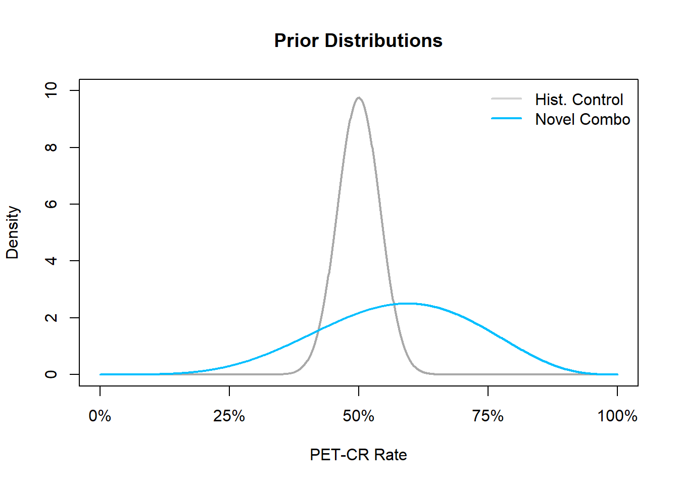
In this figure, we see that the density of the prior for the historical control is greatly concentrated in the area of the observed PET-CR rate while the prior for PET-CR rate of the novel combination is more dispersed across many potential PET-CR rates indicating a higher level of prior uncertainty.
Now, we can update our posterior uncertainty about the PET-CR rate for the novel combination via calculating the posterior distribution. Recall that our prior distribution for the novel combination PET-CR rate is a \(\text{Beta}\)(5.75, 4.25), and the data likelihood, conditional on the PET-CR rate, follows a binomial likelihood and thus, due to conjugacy, the posterior distribution will also follow a Beta distribution with updated parameters based on the observed data. For example, if after running the trial for the novel combination we were to observe 55 responders out of a total of 80 patients, i.e.,
n.samp <- 80   # Sample size of the 1b trial
n.rsp <- 55    # Number of responders
In this case, we have a PET-CR rate of 68.75%, then our posterior updating based on the prior distribution and observed data would lead to a \(\text{Beta}\)(60.75, 29.25) posterior distribution for the novel combination PET-CR rate.
xx <- seq(0, 1, .001)
dens.control <- dbeta(xx, control.shape1, control.shape2)
dens.post <- dbeta(xx, prior.shape1 + n.rsp, prior.shape2 + n.samp - n.rsp)
plot(xx, dens.control, type = "l", lwd = 2, col = "darkgrey", axes = FALSE,
     xlab = "PET-CR Rate", ylab = "Density", ylim = c(0, 10),
     main = "Posterior Distributions")
lines(xx, dens.post, lwd = 2, col = "deepskyblue")
axis(1, seq(0, 1, .25), c("0%", "25%", "50%", "75%", "100%"))
axis(2)
box()
legend("topright", c("Hist. Control", "Novel Combo"), lwd = 2, lty = 1,
       col = c("darkgrey", "deepskyblue"), bty = "n")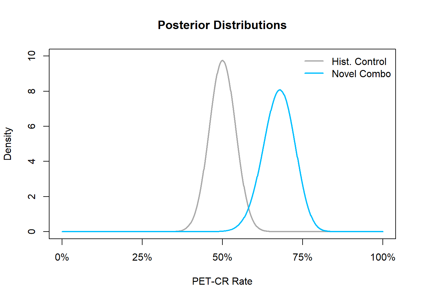
In this figure, we see that the posterior distribution is much more peaked than the prior distribution, reflecting the fact that once we have observed data, our uncertainty about the true PET-CR rate in the novel combination should diminish. Once the posterior distribution is obtained, the user can use the postprob() command to make posterior probability calculations about the PET-CR rate for either the novel combination or historical control. For example, the user could calculate the probability that the PET-CR rate is greater than 60%, i.e., \(\mathbb{P}(P_E > 0.6 \, \vert\, x)\), by issuing the following command:
postprob(x = n.rsp, n = n.samp, p = 0.6, parE = c(prior.shape1, prior.shape2))[1] 0.9322701Here the result indicates that there is a 93.23% probability that the PET-CR rate for the novel combination is above 60%.
Operating Characteristics
Similarly, the user may be interested in estimating the frequentist probability that a clinical trial is stopped for efficacy or futility, conditional on true values of the response rate. These calculations need to take into account in particular interim looks at the data before reaching the final sample size of the trial. Hence, the calculations are difficult to perform in a closed manner. However, we can resort to Monte Carlo calculation, which means that we simulate a very large number of trials and estimate with high precision the frequentist probabilities of interest. These are the key operating characteristics of the trial design.
For example, we may be interested in a conducting a single arm phase Ib trial where interim analyses will be planned once we have accrued 10, 20 and 30 patients (30 being the maximum number of patients we will accrue). We declare efficacy early, at the interim looks, if the posterior probability that the observed response rate, \(p_E\), is greater than a predefined efficacy threshold, \(p_1 = 30\%\), exceeds some upper probability threshold \(t_U=80\%\), i.e., \[ \mathbb{P}(p_E>p_1)>t_U. \] Likewise, we declare futility early if the the posterior probability that the observed response rate, \(p_E\), is less than some predefined efficacy threshold, \(p_0=20\%\), is larger than some lower probability threshold \(t_L=60\%\), i.e., \[ \mathbb{P}(p_E<p_0)>t_L. \] Following the usual Bayesian framework, we need to specify a prior distribution for the unknown response rate \(p_E\) and so we place a \(\text{Beta}(1, 1)\) prior for our unknown response rate \(p_E\).
Furthermore, we may wish to examine the operating characteristics of this design in the scenario that the true response rate, \(p\), is equal to 40% – so in a scenario where we would like to declare efficacy. In order to calculate the operating characteristics using 10^{4} (parameter ns) simulated trials, we issue the following command:
set.seed(4) # Used for reproducibility
results = ocPostprob(nn = c(10, 20, 30), p = 0.4, p0 = 0.2, p1 = 0.3, tL = 0.6,
 tU = 0.8, parE = c(1, 1), ns = nsim)
results$oc
ExpectedN PrStopEarly PrEarlyEff PrEarlyFut PrEfficacy PrFutility
[1,] 19.119 0.6722 0.6195 0.0527 0.7598 0.054
PrGrayZone
[1,] 0.1862Here the object results is a list, which stores the operating characteristics of running the simulations inside the element oc. From our simulations we have that the expected number of patients in the trial, after stopping for either efficacy or futility, is 19. Furthermore, 67% of the simulated trials stopped early at the interim analyses. Of these 10^{4} trials, 61.95% declared early efficacy while 5.27% of them were stopped early for futility. However, combining the trials that did and did not stop early, 75.64% of have declared efficacy while 5.4% of have declared futility. These percentages do not sum up to 100% because of the 10^{4} simulated trials 18.62% would not have been declared as efficacious or futile by the time the maximum sample size of 30 patients had been reached – i.e., they fell into the grayzone.
Difference in Posterior Distributions
Now, given the UNICYCLE framework, the user may be interested in showing that the novel combination is superior to the historical control when comparing PET-CR rates. In order to make such a comparison, we can make use of the dbetadiff() function to compute the distribution of the difference in PET-CR rates between the novel combination and the historical control. Returning to the previous example, recall that we placed a \(\text{Beta}\)(5.75, 4.25) prior on the PET-CR rate for the novel combination, and observed 55 responders out of 80 patients in the novel combination, as well as 75 responders out of 150 patients in the historical control. These observed PET-CR rates led to a \(\text{Beta}\)(60.75, 29.25) and a \(\text{Beta}\)(75, 75) posterior distribution for the novel combination and historical control PET-CR rates, respectively.
Based on our learning endpoint, we may believe that seeing a difference in PET-CR rates greater than some threshold, say for example 15%, may indicate a meaningful improvement in PFS for the novel combination over the historical control. Defining the difference in PET-CR rates to be \(\Delta=\text{(Combo Response) - (Control Response)}\), we may ultimately be interested in making probabilistic calculations such as \(\mathbb{P}(\Delta>15\%)\) or \(\mathbb{P}(\Delta\leq 5\%)\) because these calculations may be informative for Go and No Go decisions.
delta1 <- 0.15
delta2 <- 0.05
For example, if \(\mathbb{P}(\Delta>\) 15 \(\%)\) or the \(\mathbb{P}(\Delta\leq\) 5 \(\%)\) is large, then we may decide to declare a go or no go, respectively. Consider a probability exceeding 60% to be large, then following the same example as above, we could evaluate the following go/no go criteria based on the distribution of the difference in PET-CR with the following code:
myPlotDiff(c(prior.shape1 + n.rsp, prior.shape2 + n.samp - n.rsp),
           c(control.shape1, control.shape2), delta1, delta2, 1, 0,
xlab = "(Combo Response) - (Control Response)")
legend("topright", c("Prob. of No Go","Prob. of Go"), pch = 15,
col = c("red", "green"), bty = "n")
arrows(.5, 2, .22, 1, lwd = 2)
text(.5, 2.2, expression("Prob" * (Delta > + 15*"%")))
arrows(-.25, 2, 0, .2, lwd = 2)
text(-.25, 2.2, expression("Prob" * (Delta < + 5*"%")))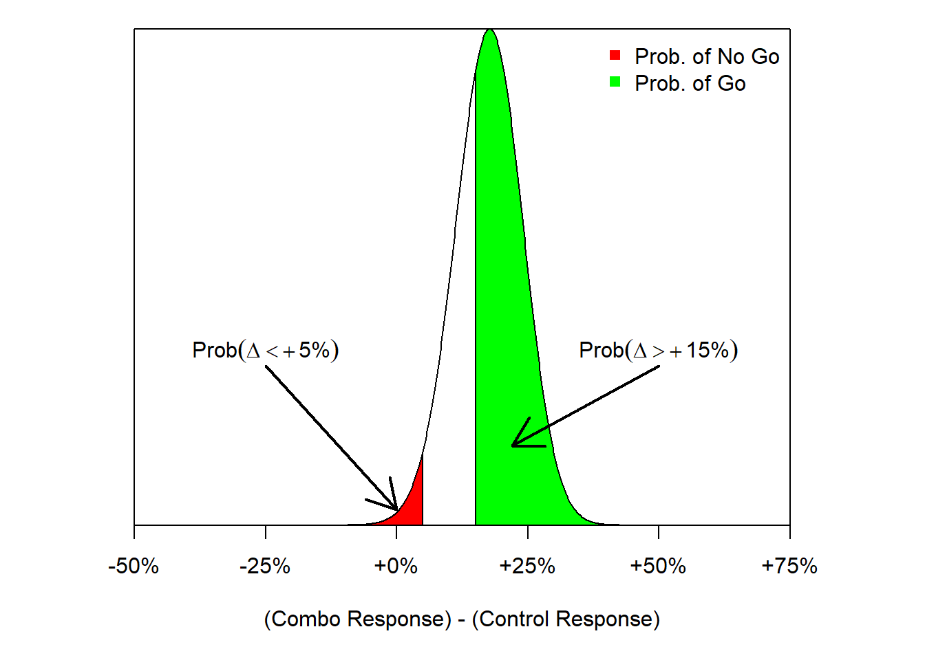
In this figure, we see that the probability of a go decision (shaded green) is much larger than the probability of a no go decision (shaded red). In fact, we can calculate those exact probability values of a go/no go decision with the following commands:
pbetadiff(delta2, parY = c(prior.shape1 + n.rsp, prior.shape2 + n.samp - n.rsp),
          parX = c(control.shape1, control.shape2)) ## NO Go
[1] 0.026845421 - pbetadiff(delta1, parY = c(prior.shape1 + n.rsp, prior.shape2 + n.samp - n.rsp),
parX = c(control.shape1, control.shape2)) ## Go[1] 0.6558079From our large threshold of exceeding 60%, we see that we would declare a go decision in this situation since the probability that \(\Delta\) exceeds 15% is equal to 65.58% which is larger than our 60% threshold.
On the other hand, had we observed a hypothetical situation where the number of responders was much lower, say 42 responders out of 80 patients, than we could re-run the same analysis to see how this would impact our go/no go decisions. The following code (an equivalent but longer code) re-runs the previous example but with a much lower response rate of \(42/80=52.5\%\).
n.rsp.new <- 42

parX <- c(control.shape1, control.shape2)
parY <- c(prior.shape1 + n.rsp.new, prior.shape2 + n.samp - n.rsp.new)
xx <- seq(-0.5, 0.75, 0.001)
dens <- dbetadiff(xx, parY, parX)
x.poly <- c(rev(xx), xx)
y.poly <- c(rep(0, length(xx)), dens)
idx1 <- which(x.poly < delta2)
idx2 <- which(x.poly > delta1)
plot(xx, dens, type = 'l', main = "PET-CR Comparison",
     xlab = "(Combo Response) - (Control Response)",
     ylab = "", yaxs = "i", axes = FALSE)
axis(1, seq(-0.5, 0.75, .25), c("-50%", "-25%", "+0%", "+25%", "+50%", "+75%"))
polygon(x.poly[idx1], y.poly[idx1], col = "red")
polygon(x.poly[idx2], y.poly[idx2], col = "green")
box()
legend("topright", c("Prob. of No Go", "Prob. of Go"), pch = 15,
       col = c("red", "green"), bty = "n")
arrows(.45, 2, .2, .5, lwd = 2)
text(.45, 2.2, expression("Prob" * (Delta > + 15*"%")))
arrows(-.3, 2, -.03, .9, lwd = 2)
text(-.3, 2.2, expression("Prob" * (Delta < + 5*"%")))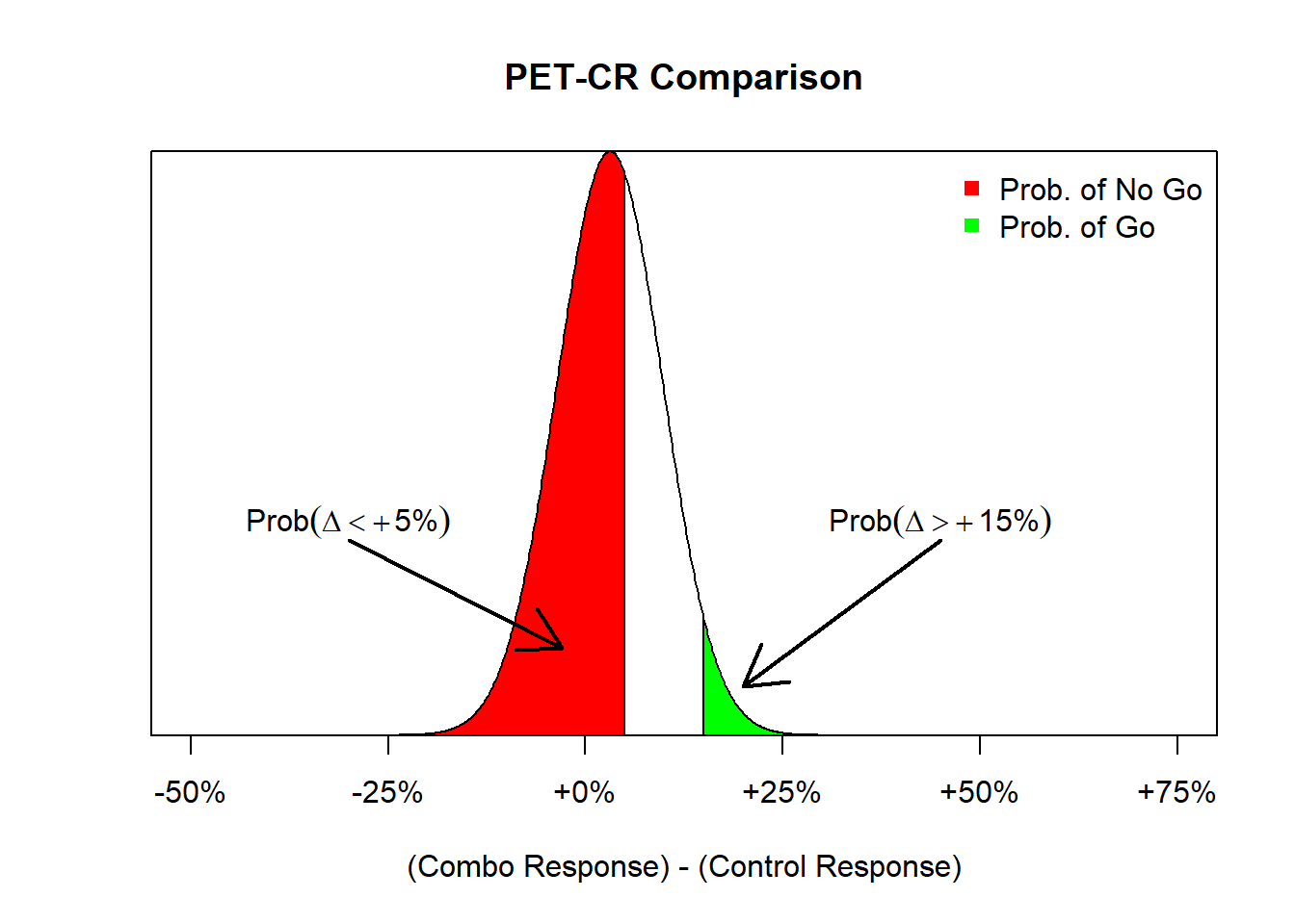
Note now that the change in response rate also affects the posterior distribution of the PET-CR rate for the novel combination group. Before the posterior distribution was a \(\text{Beta}\)(60.75, 29.25) distribution and now, due to the low observed response rate, the posterior distribution is a \(\text{Beta}\)(47.75, 42.25). Using this new posterior distribution, we obtain the following distribution of the difference in PET-CR rates between the two groups. We see that the probability of a no go decision is much higher than the probability of a go decision due to the lower response rate in the novel combination group. As before, we can execute the following commands to calculate those exact probabilities:
1 - postprobDist(x = n.rsp.new, n = n.samp, delta = delta2, parE = c(prior.shape1, prior.shape2),
                 parS = c(control.shape1, control.shape2)) ## No Go
[1] 0.6142228postprobDist(x = n.rsp.new, n = n.samp, delta = delta1, parE = c(prior.shape1, prior.shape2),
parS = c(control.shape1, control.shape2)) ## Go[1] 0.03532739Thus, there is a 61.42% chance that the novel combination results in a less than 5% improvement in PET-CR rates relative to the historical control, and hence a no go decision would be declared.
Predictive Probability Design
This example aims to illustrate the usage of predictive probabilities (PP) to conduct interim analyses (the basic PP design). The single arm 1L DLCBL combo trial which was discussed in the previous section is used in this section as well. Besides, this section also includes a simulation study to evaluate the operating characteristics of the study design.
Similar to the previous example, it has been hypothesized that a 15% absolute increase of PET-CR may predict a meaningful clinical benefit for 1L DLBCL patients. Thus the goal of the trial is set to evaluate the PET-CR rate \(P_{combo}\) by testing the hypothesis \(H_0: P_{combo} \leq P_{control}+15\%\) versus \(H_A: P_{combo} > P_{control}+15\%\). Thus let’s further determine that, when the sample size reaches the maximum, the study is to declare efficacy if the posterior probability of \(P_{combo} > P_{control}+15\%\) is greater than a threshold \(\theta_T=0.6\). Otherwise, the study is to declare futility.
Here, it is assumed that 2 interim analyses are planed at 25 and 40 patients along with a final analysis at 80 patients to evaluate both efficacy and futility. The study stops at interim when
- Efficacy stop if \(PP>\phi_U\)
- Futility stop if \(PP<\phi_L\)
where we set \(\phi_U=0.8\) and \(\phi_L=0.2\) for illustration.
Please be aware, there will be no “gray zone” in terms of decision making at the final analysis when using the the basic PP design.
Predictive Probability Calculation
To calculate the predictive probability when comparing two distributions (treatment vs. SOC), the predprobDist() function can be used. In order to perform the calculation, the maximal number of patient (80), a Beta prior of the treatment arm (\(\text{Beta}\)(5.75, 4.25)), a Beta posterior distribution of the SOC arm (\(\text{Beta}\)(75, 75)) are required. For instance, if there are 18 PET-CR at the first interim analysis (n=25), the predictive probabilities can be calculated by
# PP
predprobDist(x = 18, n = 25, Nmax = n.samp, delta = delta1, thetaT = 0.6,
             parE = c(prior.shape1, prior.shape2), parS = c(control.shape1, control.shape2))[1]
[1] 0.5755374In this case, study will continue since PP, 57.55%, does neither exceed 80% nor fall below 20%.
Operating Characteristics Evaluation
Before the phase Ib trial starts, users may want to evaluate the design operating characteristics at an assumed true PET-CR rate of the combo trial. The ocPredprobDist() function allows such an evaluation under a single scenario of true response rate. The following code assumes a true PET-CR rate of 75%. The planed interim and final looks are at 25, 40 and 80 patients which is entered as a vector in the nn argument. p is the true PET-CR rate we assumed, and we are targeting for a delta improvement over control (delta ranges from 0 to 1). tT is the threshold for the probability to be above control + delta at the end of the trial, and phiL and phiU are the lower and upper thresholds on the predictive probability, respectively. Same as the notations in the predprobDist() function, parE and parS are the place to enter beta parameters for the prior on the treatment and control proportion, respectively. Although a larger number of trials can be generated to evaluate the scenario, nsim <- 100 is used here for the purpose of illustration.
# with 100 simulated trials, assume true PET-CR rate of the combo trial is 40%
set.seed(4)
nsim <- 100
res1 <- ocPredprobDist(nn = c(25, 40, 80), p = 0.75, delta = delta1, tT = 0.6, phiL = 0.2, phiU = 0.8,
parE = c(prior.shape1, prior.shape2), parS = c(control.shape1, control.shape2), ns = nsim)
res1$oc
ExpectedN PrStopEarly PrEarlyEff PrEarlyFut PrEfficacy PrFutility
[1,] 44.4 0.71 0.6 0.11 0.87 0.13
PrGrayZone
[1,] 0According to the simulation result, the expected sample size of the trial is 44.4. 87% of the simulated trials declare efficacy and the rest 13% of trials declare futility. In terms of early stopping, 71% of the simulated trials stop at interim. Among those, \(60\%/71\%=84.5\%\) trials stop for efficacy, and \(11\%/71\%=15.5\) trials stop for futility.
Usually, more than one true scenario will be evaluated. The following figure summarizes the operating characteristics among different true PET-CR rate from 10% to 80%. Y axis is the percentage of trials that return a efficacy/futility decision. When true rate is low comparing to the response rate of control+delta, a efficacy decision is considered as a type I error, and when true rate is relatively high comparing to the control+delta, a futility decision is considered as a type II error.
set.seed(4) # Used for reproducibility
p_par <- seq(0.1, 0.9, by = 0.1)
Mysim <- sapply(p_par, function(x){
  res <- ocPredprobDist(c(25, 40, 80), x, delta = delta1, tT = 0.6, phiL = 0.8, phiU = 0.2,
                        parE = c(prior.shape1, prior.shape2),
                        parS = c(control.shape1, control.shape2), ns = nsim)
  return(res$oc)
})
peffbp <- Mysim[5, ]
pfutbp <- Mysim[6, ]
par(mar = c(5, 4, 1, 1) + .1)
plot(c(0, 1), c(0, 1), type = 'n', xlab = "True Rate", ylab = "Pr(Decision)")
grid()
lines(p_par, peffbp, lwd = 5, col = "green")
lines(p_par, pfutbp, lwd = 5, col = "red")
legend(.1, .6, lwd = 5, col = c("green", "red"), cex = .75,
       c("Efficacy Decision", "Futility Decision"))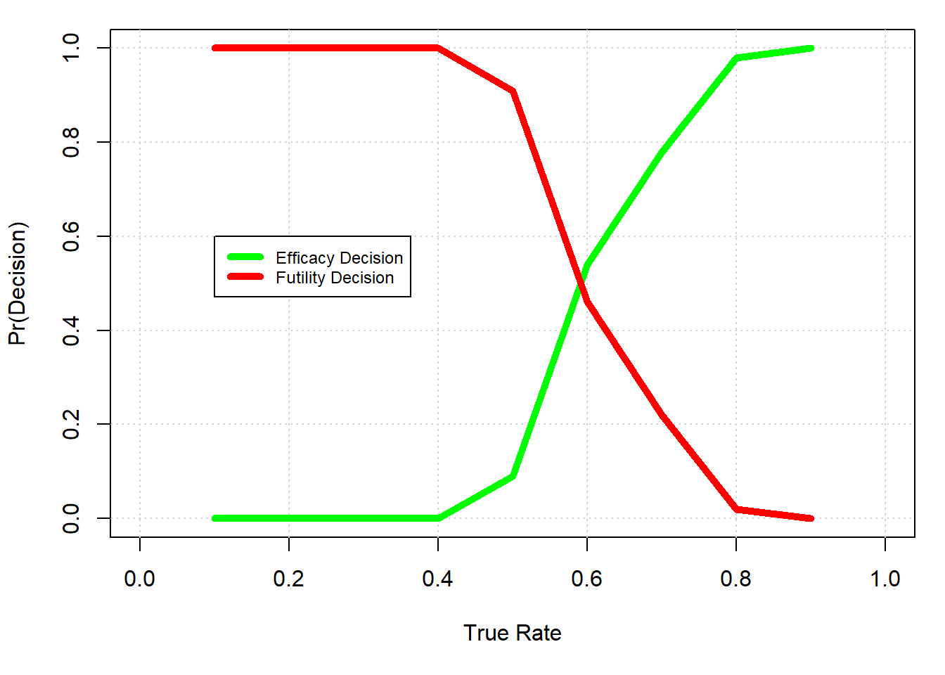
Advanced predictive probability design
This extension example shows a way to use predictive proabilities (PP) to conduct interim analyses allowing gray zones at the final analyses, i.e. trial results where neither efficacy nor futility decisions are made are possible. Such a final analysis design was used in the 1L DLBCL example from the UNICYCLE slide deck, of which the basic PP design used is not suitable for the related interim analyses, but the advanced predictive probability design should be used.
One advantage of such a design is that it allows an option of further evaluation on additional clinical endpoints or PD markers when the decision falls into the gray zone. Moreover, a seperate delta can be specified for the futility decision to represent a “pool clinical improvement”, which makes it a more flexible decision rule.
Similar to the previous example, the goal is to evaluate the PET-CR rate \(P_{combo}\) by testing the hyoithesis \(H_0: P_{combo} \leq P_{control}+15\%\) versus \(H_A: P_{combo} > P_{control}+15\%\) for efficacy. And the futility checks are conducted by testing the hyoithesis \(H_0: P_{combo} \geq P_{control}+5\%\) versus \(H_A: P_{combo} < P_{control}+5\%\). Here, we assume that 2 interim analyses are planed at 25 and 40 patients along with a final analysis to evaluate both efficacy and futility.
Thus at the final analysis:
- The design is to declare efficacy if the posterior probability of \(P_{combo} > P_{control}+15\%\) is greater than a threshold \(\theta_{U}=0.6\) (event A)
- The design is to declare futility if the posterior probability of \(P_{combo} < P_{control}+5\%\) is greater than a threshold \(\theta_{F}=0.6\) (event B)
\(\theta_{U}\) and \(\theta_{F}\) are the thresholds set for the posterior probabilities at the final analysis. 60% is assumed for both of the parameters.
In addition, we assume the study stops at interim when
- Efficacy stop if \(PP(\text{event A})>\phi_U\)
- Futility stop if \(PP(\text{event B})>\phi_F\)
where \(\phi_U=\phi_F=0.8\) for illustration. \(\phi_F\) and \(\phi_U\) are independent thresholds and can be set to unequal values depending on the need of users.
Predictive Probability Calculation
The following code shows how to utilize the predprobDist() function to calculate the PPs, if there are 18 PET-CR at the first interim analysis:
# PP(event A)
ppa <- predprobDist(x = 18, n = 25, Nmax = n.samp,
                    delta = delta1,
                    thetaT = 0.6,
                    parE = c(prior.shape1, prior.shape2),
                    parS = c(control.shape1, control.shape2))[1]
ppa
[1] 0.5755374# PP(event B)
ppb <- 1-predprobDist(x = 18, n = 25, Nmax = n.samp,
delta = delta2,
thetaT = 1 - 0.6,
parE = c(prior.shape1, prior.shape2),
parS = c(control.shape1, control.shape2))[1]
ppb[1] 0.01368629According to the result, study will continue since neither PP(event A), 57.6%, nor PP(event B), 1.4% exceed \(\phi_U=\phi_F=80\%\).
Operating Characteristics Evaluation
To evaluate the design operating characteristics at an assumed true PET-CR rate of the combo trial, the ocPredprobDist() function can be used for the advanced PP design as well. To do so, additional arguments, such as deltaFu, tFu and phiFu need to be specified. Also, the phiL argument has to be skipped. To evaluate a scenario with a true response rate of \(75\%\), the following code can be used:
#with 100 simulated trials, assume true PET-CR rate of the combo trial is 40%
set.seed(4) #Used for reproducibility
res1 <- ocPredprobDist(nn = c(25, 40, n.samp), p = 0.75,
          delta = delta1, deltaFu = delta2,
          tT = 0.6, tFu = 0.6,
          phiU = 0.8, phiFu = 0.8,
          parE = c(prior.shape1, prior.shape2), parS = c(control.shape1, control.shape2), ns = nsim)
res1$oc
ExpectedN PrStopEarly PrEarlyEff PrEarlyFut PrEfficacy PrFutility
[1,] 50 0.6 0.6 0 0.94 0
PrGrayZone
[1,] 0.06The number of simulation is 100 here to reduce the computational time of the code. However, user may want to increase the number to 10000 or higher to generate a more stable result.
Comparing to the example in previous section, there could be a gray zone at the final analysis. According to the simulation result, 6% of the simulated trials declared neither efficacy or futility at the final analysis (i.e. gray zone). The expected sample size, which is 50, tends to be higher than the previous example. 94% of the simulated trials declare efficacy, and \(60\%/94\%=63.8\%\) of them stop at interim. Besides, none of the simulated trial stop for futility.
Similar simulation analyses can be conducted for different assumed true PET-CR rates other than 75%, to have a more complete picture of the operating characteristics.
Conceptual differences between DDCP and predictive probabilities
Although both approaches intend to quantify the probability of success, they have different assumptions and applications. In this section, we provide a comparison of the conceptual differences between DDCP and the predictive probability framework. DDCP is about computing probabilities of success of trials based on assurance, see successR’s methodology tutorial. Predictive probabilities on the other are based on a positive conclusion (rejecting the null hypothesis) should the trial be conducted to the maximum planned sample size. A high level comparison is provided in the following table.
In general, DDCP and PP are two different approaches based on different assumptions with different properties and interpretations.
| Comparison | UNICYCLE | DDCP |
|---|---|---|
| Questions to answer | quantify probability to meet ‘miniTPP’ (designed for ph1b trial) given entire prior knowledge about effect size | quantify probability to beat minimal or target product profile in Phase 2 or 3 given entire prior knowledge about effect size |
| Trial of interest | Ph1b single arm trials | typically RCTs, but in theory any normally distributed test statistic allows for use of framework |
| Endpoint types | Binary | binary, continuous, time-to-event |
| Common endpoints | ORR | response proportion difference, mean difference, PFS, OS, … |
| Update after interim | Yes | Yes |
UNICYCLE: predictive probability
The predictive probability (PP) of trial success is defined to be the expected posterior probability of meaningful treatment effect, given the possible future outcome outlook and the data accumulated so far. That is,
\[ \mathbb{E}( \text{posterior of clinically meaningful effect} \, \vert \, \text{every possible future outcome}) \]
Key features of the predictive probability (PP) approach implemented in UNICYCLE:
PP approach mimics the clinical decision making process based on accumulating trial data.
Based on the interim data, PP is obtained by calculating the probability of a positive conclusion (rejecting the null hypothesis) should the trial be conducted to the maximum planned sample size.
PP evaluates the chance that the trial will show a conclusive result at the end of the study, given the current information.
Conceptually, PP can be considered as the weighted averages (by the posterior) of the conditional powers across the current probability that each success rate is the true success rate.
At intermin looks of data, PP can be used for early determination of meaningful clinical benefits.
At final analysis, PP can be used to declare futility, efficacy, or a gray zone that further evaluations are needed.
The decision to continue or to stop the trial can be made according to the strength of predictive probability.
Both a basic PP design and a more advanced PP design are available for different study needs.
See Berry et al. (2011) for more details.
successR: DDCP
The data-driven conditional probability (DDCP), also known as assurance, is a framework to quantify the probability to beat the minimal or target product profile in Phase 3 given the entire prior knowledge we have about the effect size prior to Phase 3. A detailed introduction is available here.
References
For more details for the example in Section 7, see phase1b package vignette prepared by Tony Pourmohamad, Jiawen Zhu, and Daniel Sabanes Bove.
References
Berry, Scott M., Bradley P. Carlin, J. Jack Lee, and Peter Müller. 2011. Bayesian Adaptive Methods for Clinical Trials. Vol. 38. Chapman & Hall/CRC Biostatistics Series. Boca Raton, FL: CRC Press.