# Load bpp
library(bpp)

# load rpact
library(rpact)Compute assurance at the design stage of a clinical trial: continuous endpoint
Purpose
This document provides code to compute assurance at the design stage of a clinical trial for a continuous primary endpoint measured at a specific timepoint (so not longitudinal!). We mimick the example provided in adaptr.
We have designing a Phase 3 trial in mind, but the concepts are equally well applicable when designing a Phase 2 trial. In the latter case, the success criterion might be somewhat different.
Terminology
In what follows when we talk about “effect” we always refer to actual effect, i.e. not standardized.
Setup
Load packages:
Our trial of interest
We assume that we plan a 1:1 randomized trial for a continuous endpoint, so the effect measure we are interested in is the mean difference between two arms. We further assume the trial will have one interim analysis after 50% of information. We start with defining the parameters of this pivotal trial. Note that the success probability part in bpp is parametrized such that we always look at the probability \(P(\widehat \delta_\text{fin} \le \delta_\text{suc})\), see general methodology. However, the bpp package contains a wrapper function bpp_continuous for the scenario with “higher mean is better” which we use here.
# ---------------------------------------------------
# specifications of the pivotal trial
# ---------------------------------------------------

# set up a group-sequential design with an interim after 50% of information
# significance levels at final analysis
design <- getDesignGroupSequential(sided = 2, alpha = 0.05, beta = 0.2,
                                   informationRates = c(0.5 ,1),
                                   typeOfDesign = "asOF")

# number of patients needed per arm
delta <- 10
stDev <- 24
sampleSize <- getSampleSizeMeans(design, alternative = delta, stDev = stDev)
n1 <- ceiling(sampleSize$numberOfSubjects1[2, 1])
n2 <- ceiling(sampleSize$numberOfSubjects2[2, 1])
c(n1, n2)
[1] 92 92# MDD at final
mdd <- sampleSize$criticalValuesEffectScaleUpper[2, 1]
mdd[1] 7.023506Define the prior distribution
As a next step we define the parameters of the prior density \(q(\theta)\). For a discussion of aspects of prior choice also see the tutorial on choice of prior.
Normal prior
# ----------------------------------
# mean and sd of Normal prior:
# ----------------------------------
priormean <- 12.3

# standard error of that mean difference
sig1 <- 26.1
n1p <- 25
sig2 <- 33.6
n2p <- 25
sd0 <- sqrt(sig1 ^ 2 / n1p + sig2 ^ 2 / n2p)
sd0
[1] 8.509219The above prior could e.g. result from a Phase 2 trial with observed mean difference of 12.3 (which we chose not to attenuate) and standard error 8.51. The resulting density function is depicted as red line in the figure below.
To better understand the properties of this prior we can compute a few probabilities of interest:
lims <- c(0, delta)
pnorm1 <- pnorm(lims[1], mean = priormean, sd = sd0)
pnorm2 <- 1 - pnorm(lims[2], mean = priormean, sd = sd0)
c(pnorm1, pnorm2)
[1] 0.07415999 0.60653338So the probability for the mean difference to be below 0 or above 10 amounts to 0.07 and 0.61, respectively. The prior thus allows for a 7% probability that the treatment effect may be on the harmful side.
# ----------------------------------
# parameters of pessimistic, or flat, prior:
# ----------------------------------
priormeanflat <- priormean
width1 <- 25
height1 <- 0.02
The above code specifies a more pessimistic alternative prior, see this tutorial for details on how to specify such a prior. This may potentially more accurately reflect the (absence of) knowledge about the treatment effect at the design stage or could be used as a kind of sensitivity analysis. Such a prior has e.g. been used when quantifying the success probability at the design stage in the MIRROS case study, for a time-to-event endpoint though.
To specify a pessimistic prior we retain the lower tail of the Normal prior above but move the upper tail slightly to the right, allowing for a plateau in the center of the distribution. To compute the probabilities to be below 0 or above 10 we have to integrate over the density function of the pessimistic prior. The function for this density is available in the package bpp.
flat1 <- integrate(dUniformNormalTails, lower = -Inf, upper = lims[1],
                   mu = priormeanflat, width = width1, height = height1)$value
flat2 <- integrate(dUniformNormalTails, lower = lims[2], upper = Inf,
                   mu = priormeanflat, width = width1, height = height1)$value
c(flat1, flat2)
[1] 0.2540000 0.5459999This leads to a 55% probability for the true mean difference to be above 10. The red line in the figure below illustrates this alternative prior.
par(las = 1, mar = c(4.5, 4.5, 2, 1), mfrow = c(1, 1))
xli <- priormean + 40 * c(-1, 1)
yli <- c(0, 0.05)
plot(0, 0, type = "n", xlim = xli, ylim = yli, xlab = "mean difference", ylab = "density",
     main = "Normal and pessimistic prior density for mean difference")
abline(h = 0, lty = 3)

# grid to compute densities on
thetas <- seq(-100, 100, by = 0.1)

lines(thetas, dnorm(thetas, mean = priormean, sd = sd0), col = 2, lwd = 2)
lines(thetas, dUniformNormalTails(thetas, mu = priormeanflat,
                                  width = width1, height = height1), lwd = 2, col = 3)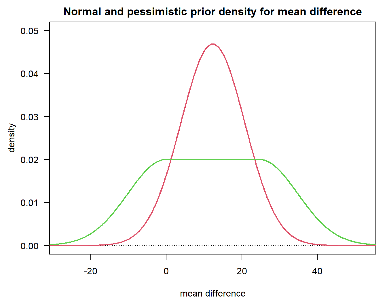
DDCP at the beginning of the trial
Having specified one or more priors together with the details of the trial of interest we can now quite easily compute the corresponding DDCP values.
# ----------------------------------
# Normal prior:
# ----------------------------------
bpp0 <- bpp_continuous(prior = "normal", successmean = mdd, stDev = stDev,
                       n1 = n1, n2 = n2, priormean = priormean, priorsigma = sd0)

# ----------------------------------
# pessimistic prior:
# ----------------------------------
bpp0_1 <- bpp_continuous(prior = "flat", successmean = mdd, stDev = stDev,
                         n1 = n1, n2 = n2, priormean = priormeanflat,
                         width = width1, height = height1)

c(bpp0, bpp0_1)
[1] 0.7165276 0.6055230Note that the arguments for bpp differ, depending on which prior you want to compute DDCP for. We find that based on our priors and the specifications for the trial of interest we get values of 0.72 and 0.61. These are our BBP values at the design stage of the trial.