# Load bpp
library(bpp)Probability of success of a clinical trial: MIRROS case study
Setup
The trial
MIRROS was a Phase 3 multicenter, double-blind, randomized, placebo-controlled trial of Idasanutlin in combination with Cytarabine compared with Cytarabine and placebo in relapsed-refractory (R/R) AML. The trial was initiated based on promising Phase 1 data and high unmet medical need for patients with R/R AML, see Reis et al. (2016). For details on the mechanism of action of Idasanutlin we refer to Tovar et al. (2006) and Vassilev et al. (2007).
At the time of the design of MIRROS, OS was the preferred endpoint. Although some patients with AML benefit from chemotherapy-based regimens, these therapies are rarely curative with the exception of stem cell transplant. For this reason, it appears sensible to incorporate a cure proportion when powering the trial. In order to account for a cure proportion the trial was powered via simulations from a mixture cure model. The technical details have all been described in Rufibach et al. (2020) and the corresponding code is available on github.
With MIRROS a Phase 3 for Idasanutlin started directly after availability of Phase 1 data, i.e. Phase 2 was integrated into Phase 3. This means a pre-planned futility interim analysis on an intermediate endpoint was planned in MIRROS. Several aspects contributed to the decision to integrate Phase 2 into Phase 3 in MIRROS:
- The very high unmet medical need in R/R AML, supporting accelerated development.
- Early phase results with Idasanutlin were considered encouraging by the sponsor.
- There exists a suitable intermediate endpoint (CR, binary) related to OS for the integration. We omit the details of the clinical assessment of CR and just mention that response-type endpoints have been previously considered suitable as intermediate endpoints, see e.g. Hunsberger et al. (2009). The timing of the IA was determined through a pre-specified number of patients that are evaluable for CR at the IA, namely 120. This number was considered suitable for making the interim decision and corresponds to the sample size of a typical randomized Phase 2 trial.
Design stage
Specifications of pivotal Phase 3 trial
We specify all the quantities of the pivotal trial, with explanations following below:
# initial PTSs
p2 <- 0.45
p3 <- 0.65

# specifications of MIRROS
alpha <- 0.05
beta <- 0.15
m1 <- 6
m2 <- 9
hr <- m1 / m2

# cure: specifiy P(CR)
p1.cr <- 0.16
or <- 2.5
odds1 <- p1.cr / (1 - p1.cr)
p2.cr <- odds1 * or / (1 + odds1 * or)

# probability to be a long-term survivor if you have CR
p.long.term <- 0.5
cure1 <- p.long.term * p1.cr
cure2 <- p.long.term * p2.cr

c(cure1, cure2)
[1] 0.0800000 0.1612903Compute the MDD assuming exponentiality:
# MDD under exp, with randomization ratio 2:1,
# based on the protocol-specified number of events
rando.control <- 1 / 3
fac <- (rando.control * (1 - rando.control)) ^ (-1)
nevents <- 275
SEs <- sqrt(fac / nevents)
za <- qnorm(1 - alpha / 2)
hrMDD <- exp(- za * SEs)
hrMDD
[1] 0.7782407The assumptions for MIRROS were:
- Two-sided significance level of \(\alpha = 0.05\).
- 2(treatment):1(control) randomization.
- 85% power to detect an overall hazard ratio (taking into account cure) of 0.67 using a standard log-rank test. This requires 275 OS events.
- The probability to be cured is assumed to be 0.08 in the control and 0.16 in the treatment arm.
- To simulate power, a mixture model for the survival function in either arm is assumed, see Rufibach et al. (2020) for details.
- For simplicity, the minimal detectable difference was computed under Exponentiality for the above hazard ratio and amounts to 0.78.
Define generic PTS
The generic PTS (and I mean “PTS” here, not “DDCP”) was defined as follows, see pRED PTS Manual, Slide 15:
- The qualitative reference value for small molecule PTS for Phase 2 amounts to \(p_{P2} = 0.35\). Since durable CRs, suggestive of OS benefit, were observed in Phase 1 \(p^g_{P2}\) was adjusted to \(p^g_{P2} = 0.45\).
- The generic value for Phase 3 PTS is \(p^g_{P3} = 0.65\).
- According to Late Stage PTS handbook if a program skips Phase 2 then PTS before start of the Phase 3 pivotal trial is received through multiplying these two values to get the Phase 3 PTS \(p_{P3}\) at trial start: \[p_{P3} = p^g_{P2} \cdot p^g_{P3} = 0.2925.\]
Tune a prior to match DDCP to fit generic PTS
Now, in order to enable the team to quantify the change in PTS in case the trial does not stop at the planned futility interim it was decided to “back-translate” this PTS value into a prior for a DDCP computation, following the steps in this tutorial. Note that PTS by itself does not offer a quantitative framework to be updated after not stopping at an interim, so resorting to DDCP is needed in this case.
To set up DDCP based on PTS for MIRROS, the following considerations were made:
- Given a Phase 3 trial is started the team was confident that the probability that the OS hazard ratio exceeds 1 should be small.
- Similarly, it was considered unlikely that the OS hazard ratio was below 0.6.
- In order not to favor an OS HR in this range the pessimistic prior introduced in Rufibach et al. (2016) was chosen, see the tutorial on prior choice.
- Finally, the prior should be tuned such that DDCP to beat the target product profile hazard ratio of 0.67 amounts to \(p_{P3} = 0.29\).
The pessimistic prior is introduced in Rufibach et al. (2016). A discussion why such a prior might be preferred over a Normal prior is provided in the tutorial on choice of prior. The parametrization in the function dUniformNormalTails in the package bpp that is used below is slightly different from the paper. Note that when considering the hazard ratio the prior has to be parametrized on the log-scale. We have four parameters that we need to set:
ea <- 0.6
eb <- 1
a <- log(ea)
b <- log(eb)
width <- b - a

priormean <- (a + b) / 2
exp(priormean)
[1] 0.7745967- The width of the horizontal stretch. It is easiest to define this through the endpoints \(a = \log(0.6)\) and \(b = \log(1)\), respectively.
- The center of the prior: we set this here at a hazard ratio of \(\exp\Bigl(\frac{\log(0.6) + \log(1)}{2}\Bigr) = \log(0.77)\).
- As described in the tutorial on backengineering a prior we find the height of the pessimistic prior through numerical root search, such that the resulting generic PTS is \(p_{P3} = 0.29\):
# set up target function
target <- function(x, pts1, successHR, d, priorHR, propA, width){
  res <- pts1 - bpp_t2e(prior = "flat", successHR = successHR, d = d, priorHR = priorHR,
                 propA = propA, width = width, height = x)
  return(res)
}

# now find the root of this target function
height_opt <- uniroot(target, interval = c(0.1, 1.8), pts1 = p2 * p3, successHR = hr, d = nevents,
                      priorHR = exp(priormean), propA = 1 / 3, width = width)$root
height_opt
[1] 1.422807So the optimal height is \(h = 1.4228066\). These parameter choices give the following prior:
par(las = 1, mar = c(8, 6, 2, 1), mfrow = c(1, 1))
plot(0, 0, type = "n", xlim = log(c(0.5, 1.2)), ylim = c(-0.1, 2), xlab = "", ylab = "density",
     main = "")
title(expression("Pessimistic prior density "*q[0]*" for "*theta), line = 0.7)
basicPlot(leg = FALSE, IntEffBoundary = NA, IntFutBoundary = NA, successmean = NA, priormean = NA)
thetas <- seq(0.35, 7.5, by = 0.01)
lthetas <- log(thetas)
lines(lthetas, dUniformNormalTails(lthetas, mu = priormean, width = width, height = height_opt),
      lwd = 2, col = 3)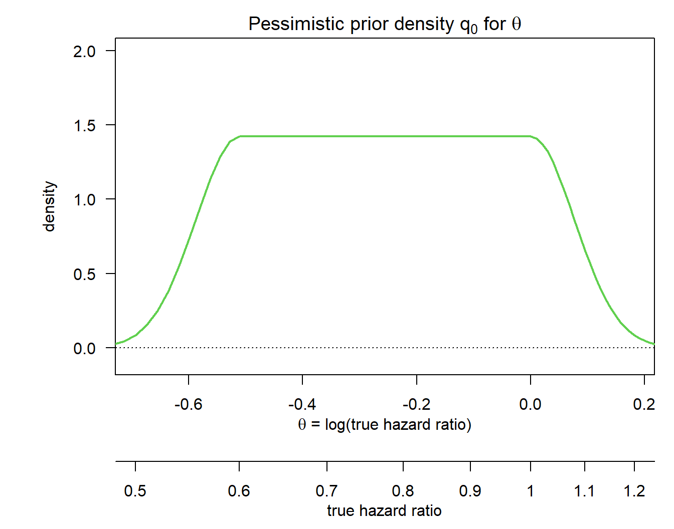
We can compute probabilities of potential interest based on this prior:
# DDCP at TPP
p_tpp <- bpp_t2e(prior = "flat", successHR = hr, d = nevents, priorHR = exp(priormean),
                 propA = rando.control, width = width, height = height_opt)

# DDCP at MDD
p_mdd <- bpp_t2e(prior = "flat", successHR = hrMDD, d = nevents, priorHR = exp(priormean),
                 propA = rando.control, width = width, height = height_opt)

c(p_tpp, p_mdd)
[1] 0.2925000 0.5066126So the design stage DDCP for MIRROS based on the above prior was indeed 29.25% to beat the TPP, as required.
Update DDCP if interim is passed
nevents_ia <- 50To mitigate the risk of directly moving from Phase 1 to Phase 3 in MIRROS a futility interim was planned after 50 OS events. The question of the LSPC at the time was then how DDCP changes as a function of the interim boundary \(\theta_{fut}\) on the log OS hazard ratio if the trial does not stop at this interim. This entails that after the interim analysis we know for the observed log hazard ratio \(\hat {\theta}_{inte}\) that \[ {\hat \theta}_{inte} \in [\theta_{eff}, \theta_{fut}] \ = \ [\log(0), \theta_{fut}]. \]
To compute these updates for both MDD and TPP we can follow the steps outlined in this tutorial.
success <- c(hr, hrMDD)
bounds_ia <- c(0.8, 0.9)
nrows <- length(bounds_ia) * length(success)
results <- matrix(NA, ncol = 5, nrow = nrows)
colnames(results) <- c("Scenario", "HR to beat at final", "DDCP at design stage",
                       "interim bound", "updated DDCP")
results[, 1] <- 1:nrows
results[, 3] <- rep(c(p_tpp, p_mdd), each = 2)

iter <- 1

v <- rep(NA, nrows)
for (i in 1:length(success)){
  success_i <- success[i]

  for (j in 1:length(success)){
    bound_j <- bounds_ia[j]

    bpp_ij <- bpp_1interim_t2e(prior = "flat", successHR = success_i, d = c(nevents_ia, nevents),
                               IntEffBoundary = 0, IntFutBoundary = bound_j, IntFixHR = 1,
                               priorHR = exp(priormean), propA = rando.control, thetas = thetas,
                               width = width, height = height_opt)

    # collect results
    results[iter, 2] <- success_i
    results[iter, 4] <- bound_j
    results[iter, 5] <- bpp_ij$"BPP after not stopping at interim interval"

    iter <- iter + 1
  }
}

# prettify and display output
results[, 2:5] <- apply(results[, 2:5], 1:2, disp, 2)
knitr::kable(results, align = "ccccc")| Scenario | HR to beat at final | DDCP at design stage | interim bound | updated DDCP |
|---|---|---|---|---|
| 1 | 0.67 | 0.29 | 0.80 | 0.48 |
| 2 | 0.67 | 0.29 | 0.90 | 0.42 |
| 3 | 0.78 | 0.51 | 0.80 | 0.73 |
| 4 | 0.78 | 0.51 | 0.90 | 0.68 |
So as an example in Scenario 4 we consider the situation where DDCP is computed to beat a hazard ratio of 0.78. At the design stage of the trial DDCP to beat this hazard ratio amounts to 0.51. If we do not stop the trial at a futility interim analysis with a pre-specified interim boundary for the OS hazard ratio of 0.90 then this DDCP increases to 0.68.
What really happened
For MIRROS the decision criteria at the interim analysis was not only based on the OS hazard ratio, but in addition also on a criterion for the odds ratio for CR. At the team the also included this criteria into the modelling to update DDCP after not stopping at the interim, using the simulation model discussed in Rufibach et al. (2020), with code available on github. If you are interested in the details reach out to kaspar.rufibach@roche.com.
Outcome of MIRROS
The futility interim for MIRROS was passed but the trial was stopped after an interim analysis at 80% of information.
References
Hunsberger, S., Y. Zhao, and R. Simon. 2009. “A comparison of phase II study strategies.” Clin. Cancer Res. 15 (19): 5950–55.
Reis, B., L. Jukofsky, G. Chen, G. Martinelli, H. Zhong, W. V. So, M. J. Dickinson, et al. 2016. “Acute myeloid leukemia patients’ clinical response to idasanutlin (RG7388) is associated with pre-treatment MDM2 protein expression in leukemic blasts.” Haematologica 101 (5): e185–188.
Rufibach, Kaspar, Dominik Heinzmann, and Annabelle Monnet. 2020. “Integrating Phase 2 into Phase 3 Based on an Intermediate Endpoint While Accounting for a Cure Proportion – with an Application to the Design of a Clinical Trial in Acute Myeloid Leukemia.” Pharmaceutical Statistics 19 (1): 44–58.
Rufibach, K., H. U. Burger, and M. Abt. 2016. “Bayesian Predictive Power: Choice of Prior and Some Recommendations for Its Use as Probability of Success in Drug Development.” Pharm. Stat. 15: 438–46.
Rufibach, K., P. Jordan, and M. Abt. 2016. “Sequentially updating the likelihood of success of a Phase 3 pivotal time-to-event trial based on interim analyses or external information.” J Biopharm Stat 26 (2): 191–201. http://dx.doi.org/10.1080/10543406.2014.972508.
Tovar, C., J. Rosinski, Z. Filipovic, B. Higgins, K. Kolinsky, H. Hilton, X. Zhao, et al. 2006. “Small-molecule MDM2 antagonists reveal aberrant p53 signaling in cancer: implications for therapy.” Proc. Natl. Acad. Sci. U.S.A. 103 (6): 1888–93.
Vassilev, L. T. 2007. “MDM2 inhibitors for cancer therapy.” Trends Mol Med 13 (1): 23–31.