packs.html <- c("rpact", "bpp", "tidyverse", "stringr", "knitr")
for (i in 1:length(packs.html)){
  suppressPackageStartupMessages(library(packs.html[i],
                                         character.only = TRUE,
                                         warn.conflicts = FALSE))}

# need at least bpp version 1.0.4
if(packageVersion("bpp") < "1.0.4"){stop("Please install bpp >= 1.0.4!")}PivGo gating criteria: GYM329 in obesity
Setup
Context
During 2023, GYM329 was explored as an add-on therapy to standard of care (SoC) incretins in obesity. While the current SoC provides meaningful body weight loss (~15 - 20%) around 1/3 of this comes from lean mass loss. Furthermore, weight loss is not sustained once incretin treatment is discontinued. GYM329 is an anti-myostatin “muscle preserver” which aims to address these issues when given as an add-on therapy to incretins.
In late 2023 eSPC approved the following CDP:
- Phase 1 PK trial to assess PK in individuals of higher body weight.
- Phase 2 dose finding trial.
- Series of Phase 3 trials in overweight/obese people with/without Type 2 diabetes.
While having initial discussions on CDP design, successR was one tool considered to evaluate hte potential end of Phase 2 PivGo decision criteria.
Considerations from the team
DDCP is calculated
- based on one dose level from the Phase 2 dose finding trial.
- for one Phase 3 trial, even though there will be multiple trials in the CDP.
Proposed trial designs
Phase 2
- Primary endpoint: percentage body weight loss at one year.
- 4 arm trial. 1:1:1:1 randomization to placebo and 3 active doses.
- Sample size ~50 per arm.
Phase 3
- Primary endpoint: percentage body weight loss at one year.
- 1:1 randomization to GYM329 + incretin vs. incretin alone.
Specification details are:
# trial design operating characteristics
alpha <- 0.05
beta <- 0.1
design <- getDesignGroupSequential(sided = 2, alpha = alpha, beta = beta, kMax = 1)

# assumptions for endpoint
delta <- 5
stDev <- 9

# sample size
sampleSize <- getSampleSizeMeans(design, alternative = delta, stDev = stDev)
n_perarm <- ceiling(sampleSize$numberOfSubjects1[1, 1])
mdd <- sampleSize$criticalValuesEffectScaleUpper[1, 1]
mdd
[1] 3.02874# account for assumed dropout
drop <- 0.1
nfinal <- ceiling(n_perarm / (1 - drop))
nfinal[1] 78So we use:
- 90% power for a difference between GYM329 + incretin and incretin alone of 5 percentage points (in line with the MPP).
- 2-sided significance level \(\alpha = 0.05\).
- Common standard deviation of 9 (based on literature).
- Assumed 10% drop-out per year.
These assumptions give rise to a Phase 3 trial with \(n = 78\) per arm and an MDD of 3 percentage points.
Note that these are sample size considerations based on efficacy - the trial will need to be much larger to meet safety database requirements (FDA guidance). This is why some of the conventional sample size assumptions (e.g. MPP = MDD) do not quite align for this example.
What would we need to see in Phase 2 for 60% DDCP for Phase 3?
60% DDCP was considered as one “rule of thumb” metric.
Approach 1: Vary prior mean only
Set up a range of potential prior distributions (representing the data from the Phase 2 trial) and plot.
priormean <- seq(0, 10, 0.1)
sd <- 9
n <- 50
sd0 <- sqrt(sd ^ 2 / n + sd ^ 2 / n)

x <- seq(-10, 20, by = 0.1)
dat <- matrix(nrow = length(x), ncol = length(priormean))

for (i in 1:length(priormean)){
  dat[,i] <- dnorm(x, mean = priormean[i], sd = sd0)
}

colnames(dat) <- paste0('y_', priormean)
dat <- data.frame(x, dat)

dat %>% pivot_longer(colnames(dat)[-1]) %>% ggplot(aes(x = x, y = value, colour = name)) +
  geom_line() +
  ylab('Density') +
  xlab('Delta') +
  ggtitle('Normal prior density for delta') +
  theme(legend.position = 'none')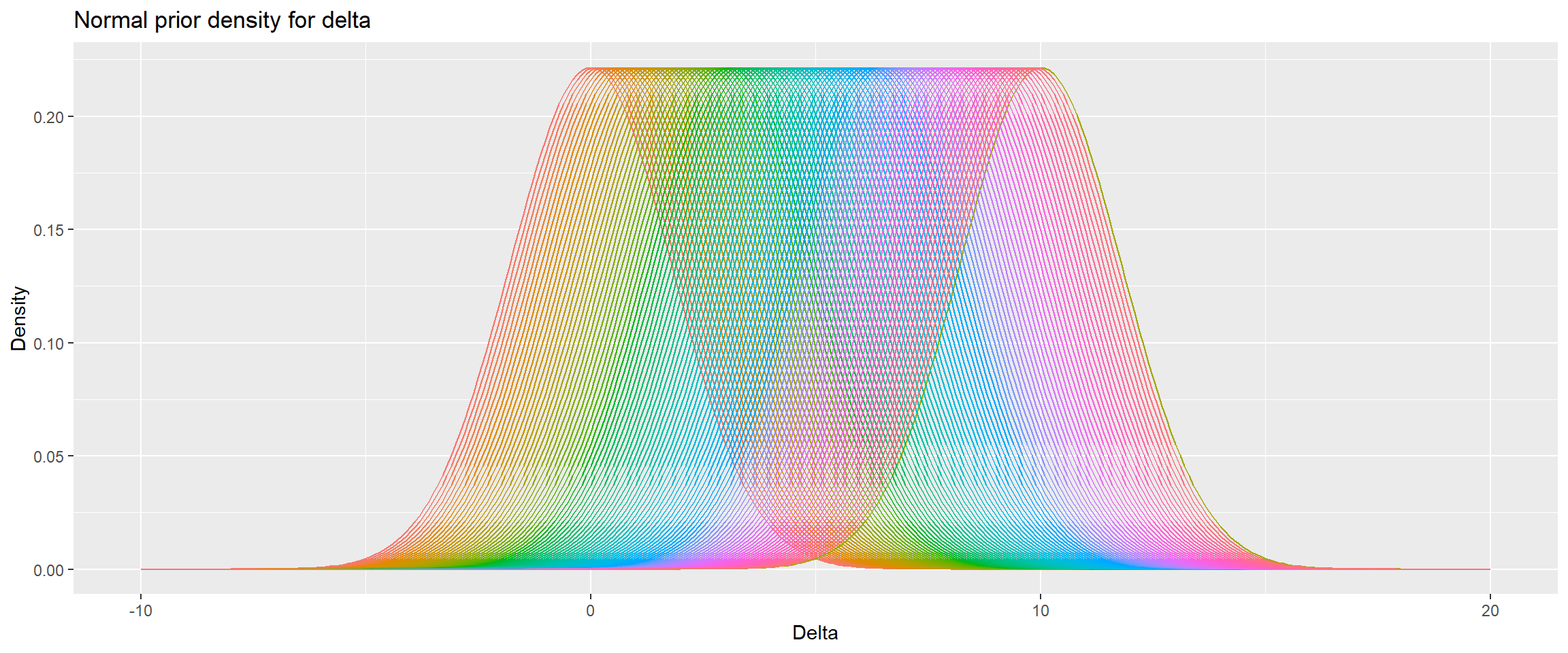
Next steps and considerations:
- Calculate DDCP for this range of priors and plot against a success threshold. For simplicity, we are only presenting one success threshold here (delta of 5 percentage points) although several were considered in reality.
- It may be typical to tie “success” to achieving the Phase 3 MDD, but given the large Phase 3 trials we will need to perform the success threshold is driven by clinical meaningful difference and minimum needed for regulatory approval per FDA guidance.
# Specify success threshold
success_thresh <- 5

# success DDCP
pts1 <- 0.6

# Set up results dataframe
ddcp_dat <- data.frame('Delta' = rep(priormean, length(success_thresh)),
                       'Success' = rep(success_thresh, each =length(priormean)),
                       'DDCP' = rep(NA, length(priormean)*length(success_thresh)))

# Calculate DDCP
for (i in 1:nrow(ddcp_dat)){
  ddcp_dat$DDCP[i] <- bpp_continuous(prior = "normal", successmean = ddcp_dat$Success[i],
                                     stDev = stDev,
                                     n1 = n_perarm, n2 = n_perarm,
                                     priormean = ddcp_dat$Delta[i], priorsigma = sd0)
}

# Pull out decision criteria for DDCP = 60%
decision_criteria_delta <- ddcp_dat$Delta[round(ddcp_dat$DDCP, 2) == pts1]

# Plot
ddcp_dat %>% ggplot(aes(x = Delta, y = DDCP, colour = factor(Success))) +
  geom_line() +
  xlab('Phase 2 delta') +
  ggtitle(paste('Decision criterion to target for 60%', pts1, ' DDCP', seP = "")) +
  geom_segment(y = 0.6, yend = 0.6, x = 0,
               xend = decision_criteria_delta[length(success_thresh)],
               linetype = 'dashed', colour = 'red') +
  geom_segment(data = data.frame(decision_criteria_delta),
               aes(y = 0, yend = 0.6, x = decision_criteria_delta,
                   xend = decision_criteria_delta), linetype = 'dashed',
               colour = 'red') +
  scale_y_continuous(breaks = seq(0, 1, 0.2)) +
  scale_colour_discrete(name = 'Phase 3 delta',
                        labels = paste0(success_thresh, '%')) +
  annotate(geom = "text", x = max(priormean)-1.5, y = 0.1,
           label = paste0('Decision criterion (', success_thresh, '%) = ',
                          decision_criteria_delta, '%', collapse = '\n')) +
  labs(caption = paste('Prior based on incretin alone vs.
        GYM329 + incretin with 50 pts per arm.
        Endpoint = % body weight loss at 1 year.
        SD for % body weight loss = ', stDev, '.
        Phase 3 sample sized based on ', 100 * (1 - beta),
        '% power for ', delta, '% delta', sep = ""))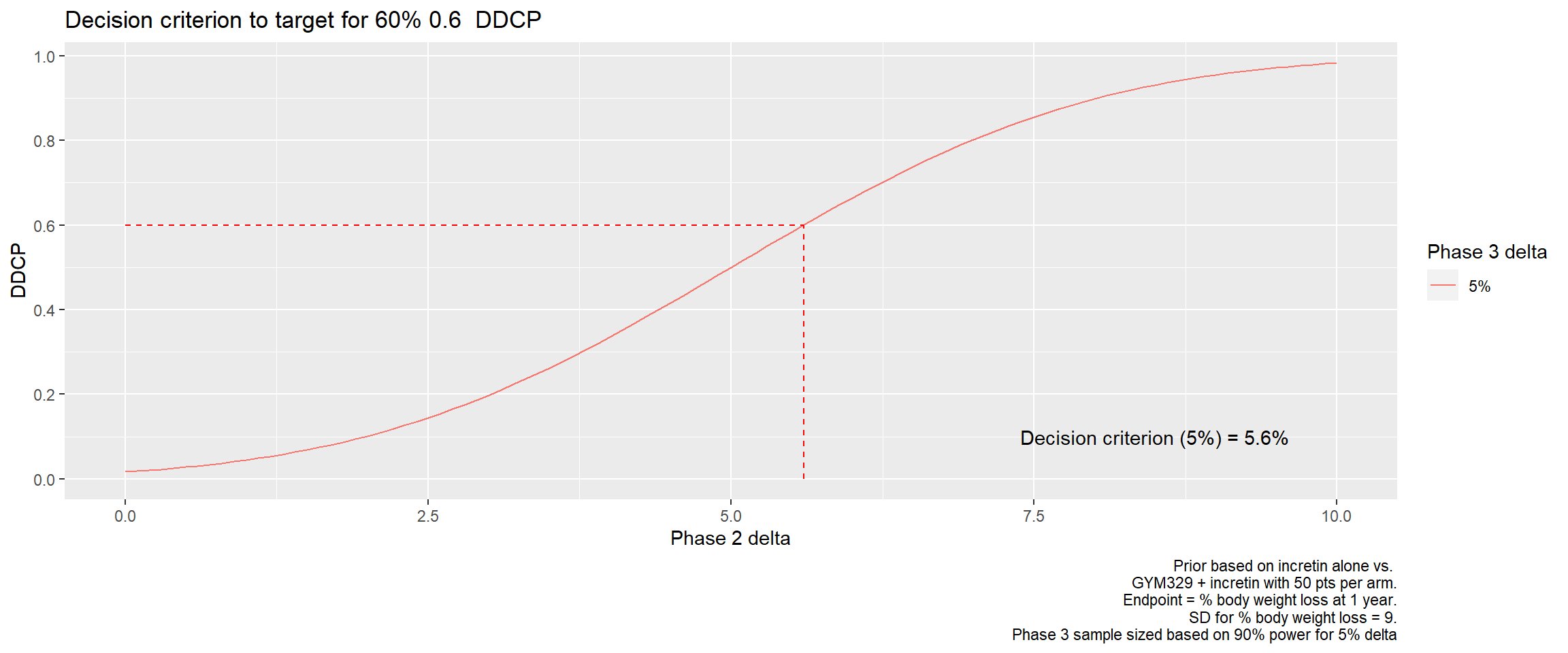
Approach 2: Vary prior sample size to reflect uncertainty
# Guess sample size that the prior knowledge should be 'worth'
n0 <- c(10, 20, 30, 40, 50)

# SD of difference for Phase 3
finalSE <- sqrt(stDev ^ 2 / n_perarm + stDev ^ 2 / n_perarm)

# Success criteria
successmean <- 5

# Set up a dataframe to store all this and calculate SD of difference for Phase 2
calc_data <- data.frame('n0' = rep(n0, length(successmean)),
                        successmean = rep(successmean, each = length(n0))) %>%
                        mutate(sd0 = sqrt(stDev ^ 2 / n0 + stDev ^ 2 / n0))

# Find the prior means that correspond to this choice of pts1 and n0
calc_data <- calc_data %>% mutate(delta0 = successmean +
                                    qnorm(pts1)*sqrt(finalSE ^ 2 + sd0 ^ 2),
                                    delta0 = round(delta0, 3))

# Generate distributions from these priors for plotting
x <- seq(-10, 20, by = 0.1)
dat <- matrix(nrow = length(x), ncol = nrow(calc_data))

for (i in 1:nrow(calc_data)){
  dat[,i] <- dnorm(x, mean = calc_data$delta0[i], sd = calc_data$sd0[i])
}
colnames(dat) <- paste0('y_n', calc_data$n0, '_success', calc_data$successmean)
dat <- data.frame(x, dat)
my_values <- c(paste0('N = ', calc_data$n0, ', Delta = ', round(calc_data$delta0, 2)))
my_names <- colnames(dat)[-1]

# Plot and check that the calculated values back-translate to ~ 60% DDCP
colours <- palette(rainbow(length(n0)))
dat <- dat %>% pivot_longer(colnames(dat)[-1]) %>%
                mutate(successthresh = as.numeric(str_sub(name, -1)),
                                                   n = str_sub(name, 4,5))

for (i in successmean) {
  my_names_sub <- my_names[str_sub(my_names, -1) == i]
  my_values_sub <- my_values[my_names %in% my_names_sub]

  labels <- setNames(my_values_sub, my_names_sub)

  plot1 <- dat %>% filter(successthresh == i) %>%
    ggplot(aes(x = x, y = value, colour = name)) +
    geom_line() +
    geom_vline(aes(xintercept = successthresh),
               linetype = 'dashed', colour = 'black') +
    xlab('Delta') +
    ylab('Density') +
    theme(
      legend.position = c(.05, .95),
      legend.justification = c("left", "top"),
      legend.box.just = "left",
      legend.margin = margin(6, 6, 6, 6)
    ) +
    ggtitle(paste0('Normal prior densities (Phase 3 delta = ', i,'%)')) +
    labs(caption = paste('Based on incretin alone vs. GYM329 + incretin.
       Endpoint = % body weight loss at 1 year.
       SD for % body weight loss = ', stDev,'.', sep = "")) +
    scale_colour_manual(name = paste("Sample size and delta for DDCP = ",
                                     100 * pts1, "%", sep = ""),
                        breaks = my_names_sub,
                        labels = labels,
                        values = colours)
  print(plot1)

  # Check that these values back translate to 60% DDCP
  bpp_back <- bpp_continuous(prior = "normal",
                 successmean = i,
                 stDev = stDev,
                 n1 = n_perarm,
                 n2 = n_perarm,
                 priormean = calc_data$delta0[calc_data$successmean == i],
                 priorsigma = calc_data$sd0[calc_data$successmean == i])
  print(bpp_back)
}
[1] 0.5999903 0.6000502 0.6000471 0.5999797 0.5999874Create false decision probability plots (false go, false no go)
- False go: Go decision when drug has no effect.
- False no go: Stop decision although drug is a ‘success’.
# Consider a range of decision criteria. In this case, change from baseline delta = 0 - 10
# SD = 9
# Calculate probability of observing >= delta when true delta = 0 or true delta = 5

# Estimate pooled SD of difference, assuming prior sample size of 50
sd0 <- sqrt(9 ^ 2 / 50 + 9 ^ 2 / 50)

# Look at a range of GO criteria
max_go <- 10
x <- seq(0, max_go, 0.01)

# Calculate the corresponding probabilities of seeing >= the GO criteria,
# given a couple of scenarios
y_0 <- 1 -pnorm(x, mean = 0, sd = sd0)
y_5 <- 1 -pnorm(x, mean = 5, sd = sd0)
dat <- data.frame(x, y_0, y_5)

# Plot
decision_criteria <- '5.6'
thresholds <- dat %>% filter(x == decision_criteria)

dat %>% pivot_longer(c(y_0, y_5)) %>% ggplot(aes(x = x, y = value, colour = name)) +
  geom_line() +
  geom_vline(xintercept = thresholds[1,1], linetype = 'dashed', colour = 'black') +
  xlab('GO criterion: Observed improvement in % weight loss vs. incretin') +
  ylab('Likelihood to hit GO criterion') +
  scale_colour_manual(name = "",
                        labels = c("GYM329 is ineffective: weight loss benefit = 0%",
                                   "GYM329 is effective: weight loss benefit = 5%"),
                        values=c("red", "green")) +
  theme(legend.position = 'bottom') +
  scale_y_continuous(breaks = seq(0, 1, 0.2)) +
  scale_x_continuous(breaks = seq(0, 10, 1)) +
  ggtitle('Risk assessment for GO or NO-GO decision') +
  geom_segment(y = thresholds[1,2], yend = thresholds[1,2], x = 0,
               xend = thresholds[1,1], linetype = 'dashed', colour = 'red') +
  geom_segment(y = thresholds[1,3], yend = thresholds[1,3], x = 0,
               xend = thresholds[1,1], linetype = 'dashed', colour = 'green') +
  annotate(geom="text", x = max_go-1, y = 0.9, label = paste0(
    'False GO = ', round(thresholds[1,2]*100, 0), '%
    False NO GO (5%) = ', 100 - round(thresholds[1,3]*100, 0), '%')) +
  labs(subtitle = paste0('Decision criterion = ', decision_criteria, '%'),
  caption = 'Based on incretin alone vs. GYM329 + incretin with 50 pts per arm.
       Endpoint = % body weight loss at 1 year.
       SD for % body weight loss = 9.') +
  guides(colour=guide_legend(nrow=2,byrow=TRUE))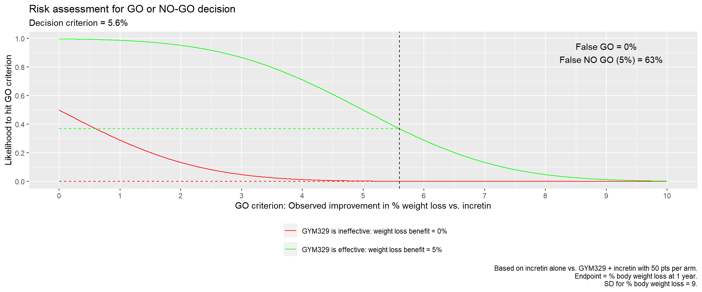
Outcome
Calculations and plots were presented to the project team to help inform a first version of the PivGo decision criteria. The DDCP calculations and first proposed PivGo rules are based on the MPP: 5.6% delta in Phase 2 for 60% DDCP for 5% delta in Phase 3.
Discussions are ongoing.