Probability of success of a clinical trial: GAZYVA case study

Author

Affiliation

Kaspar Rufibach

Methodology, Collaboration, and Outreach Group, PD DSS, Roche Basel

Published

Invalid Date

Setup

# Load bpp
library(bpp)

The Gazyva development program

Here, I only give very brief context of the entire program. I have presented on this externally before, see e.g. here for a comprehensive slidedeck.

What we have done in this program with respect to DDCP intended to be

informed through data as much as possible,
pragmatic,
tried to reflect uncertainties to some extent.

However, the fact this appears here as a case study is not intended to imply that this was the perfect way of doing this. It is an example how a team handled the challenge of continue to provide updates of DDCP throughout a big development program, using the information gained

from other trials and
from not stopping at interim analyses.

Lymphoma

Lymphomas are a group of diseases that can (could at the time) be broadly classified into:

B-cell malignancies:
- Indolent non-Hodgkin lymphoma (iNHL),
- diffuse large B-cell lymphoma (DLBCL, aggressive NHL),
- chronic lymphocytic lymphoma (CLL).

Prior to Gazyva the standard therapy for all these diseases was rituximab + chemo. The accepted primary endpoint was progression-free survival (PFS). At the time of initiation of the program it was widely believed that response (complete, CR, overall = complete + partial response, ORR) at end of chemo provides an indication of efficacy.

Gazyva

Gazyva (GA101, obinutuzumab) is a 2nd generation anti-CD20 antibody which demonstrated single agent activity in iNHL, DLBCL, CLL. The intention when kicking off the development program was to become best-in-class with superior efficacy, supposed to broadly replace rituximab. However, as the rituximab patent expiration was looming there was some risk appetite when the program was started and a fast to market strategy was chosen, moving into Phase 3 very quickly.

Trials that served as external information

The trials that informed DDCP computations were:

Gauss:
- Randomized Phase 2 trial in R/R iNHL,
- GA101 mono vs. rituximab mono,
- 149 patients, primary endpoint ORR, PFS also collected.
Two randomized Phase 3 trials:

Trial	Line	Indication	primary endpoint	1st patient randomized
CLL11	1st	CLL	PFS	April 2010
Gadolin	2nd	indolent NHL	PFS	April 2010

Trials for which DDCP needed to be computed and updated during the course of the program

DDCP updates were requested for two trials: Goya and Gallium. Key features of these trials were:

Trial	Line	Indication	primary endpoint	1st patient randomized
Gallium	1st	indolent NHL	PFS	July 2011
Goya	1st	aggressive NHL	PFS	July 2011

A futility interim analysis after \(\approx 30\%\) of information and an efficacy interim analysis after \(\approx 67\%\) of information was planned for all the four Phase 3 trials.
Interim analyses were conducted by an iDMC, i.e. the sponsor did only learn the iDMC decision (“stop” or “continue”) but not the value of the PFS hazard ratio at the interim analysis.

A framework to compute and update Bayesian predictiver power for both, Gallium and Goya, as the program evolved over time was then required.

Design stage

At the design stage the generic PTS of 0.65 was assumed for both Goya and Gallium.

Event	Goya	Gallium
First discussion of trials	0.65	0.65

Updates over time

Event 1 Q1/2011: read-out of Gauss

In Q1/2011, before Goya and Gallium randomized their first patient, Gauss read-out. Results were:

Investigator response: \(\Delta\)ORR 4.6%.
Independently-assessed response: \(\Delta\)ORR 15.2%.
PFS hazard ratio 1.07.

Based on these results, generic PTSs for Goya and Gallium were qualitatively decreased to 0.41

Event	Goya	Gallium
First discussion of trials	0.65	0.65
Update 1, Q1/2011	0.41	0.41

Event 2 Q1/2013: various results

At this time, four sources of knowledge about the effect of Gazyva became available:

CLL11: two final analyses in this 3-arm trial: Gazvya vs. standard chemo, Rituximab vs. standard chemo.
Gauss: PFS update.
Gallium: futility interim on CR passed.
Goya: futility interim on CR passed.

While these are all randomized tirals they are still different:

different primary endpoints,
different phase,
different indications.
Gauss already used for PTS computation with earlier snapshot.

So, how should we quantify all this knowledge and use it to update PTS for Goya and Gallium?

CLL11

CLL11 was a Phase 3 randomized 3-arm trial in CLL. The arms were

A: chlorambucil (C, control),
B: Rituximab + C,
C: Gazyva + C,

randomized in a 1:2:2 ratio. In Q1/2013 results of the first two comparisons, G vs. C and R vs. C based on two different snapshots (termed “Stage 1a” and “Stage 1b”), became available. The results were:

# hazard ratios
HRGvsC <- 0.14
HRRvsC <- 0.32

# number of events
nGvsC <- 123
nRvsC <- 175
nGvsR <- 151

# from the HRs of G vs. C and R vs. C we can approximate the HR of G vs. R assuming Exponentiality
HRGvsR <- HRGvsC / HRRvsC
HRCLL11 <- HRGvsR

# the standard errors for each log(HR) estimate is (note 2:1 randomization):
theta <- 1 / 3
fac <- 1 / (theta * (1 - theta))
SElogGvsC <- sqrt(1 / nGvsC * fac)
SElogRvsC <- sqrt(1 / nRvsC * fac)

# using all this we can now compute SE(log(HRGvsR)), based on the variances:
SECLL11 <- sqrt(SElogGvsC ^ 2 + SElogRvsC ^ 2)
nGvsR_computed <- 4 / SECLL11 ^ 2
nCLL11 <- nGvsR_computed

So instead of the usual variance factor of 4 for the hazard ratio when we have 1:1 randomization the factor is \((0.33 \cdot (1 - 0.33))^{-1} = 4.5\), with square root \(\sqrt(4.5) = 2.12\).

Stage 1a: \(\hat \lambda_{\mathrm{GvsC}} = 0.14\), based on 123 events. \(\mathrm{SE}(\log \hat \lambda_{\mathrm{GvsC}}) \ = \ 2.12 \cdot 123^{-1/2} \ = \ 0.19\).
Stage 1b: \(\hat \lambda_{\mathrm{RvsC}} = 0.32\), based on 175 events. \(\mathrm{SE}(\log \hat \lambda_{\mathrm{RvsC}}) \ = \ 2.12 \cdot 175^{-1/2} \ = \ 0.16\).
Assuming Exponentiality: \(\hat \lambda_{\mathrm{GvsR}} \approx \hat \lambda_{\mathrm{GvsC}} / \hat \lambda_{\mathrm{RvsC}} = 0.44\).

The standard error of \(\log \hat \lambda_{\mathrm{GvsR}} = \log \hat \lambda_{\mathrm{GvsC}} - \log \hat \lambda_{\mathrm{RvsC}}\) is then:

\[ \begin{aligned} \mathrm{SE}(\log \hat \lambda_{\mathrm{GvsR}}) \ &= \ \sqrt{\mathrm{SE}(\log \hat \lambda_{\mathrm{GvsC}})^2 + \mathrm{SE}(\log \hat \lambda_{\mathrm{RvsC}})^2 } \\ \ &= \ \sqrt{0.19 ^ 2 + 0.16 ^ 2} \\ \ &= \ 0.25 \ = \ \sqrt{4 / 64.2}. \end{aligned} \]

So backcalculating from \(\mathrm{SE}(\log \hat \lambda_{\mathrm{GvsR}})\) we find that the information on the hazard ratio G vs. R from CLL11 at this milestone is worth approximately \(64.2\) patients. Noticing that the distribution of a log(HR) can we sufficiently well approximated by Normal distributiion we can finally quantify the knowledge from CLL11 at this milestone as \(X_\mathrm{CLL11} \sim N(\log 0.44, 4 / 64.2)\). Note that G vs. R was randomized 1:1, so we again use a variance factor of 4 here.

Updated analysis from Gauss

The updated analysis for Gauss gave the following results:

# hazard ratio
HRGauss <- 0.96

# number of events and corresponding SE
nGauss <- 76
SEGauss <- sqrt(4 / nGauss)

So we quantify that information as \(X_\mathrm{Gauss} \sim N(\log 0.96, 4 / 76).\)

Gallium does not stop at futility interim

The iDMC charter for the first futility analysis in Gallium invited the iDMC to recommend continuation of the trial if the CR proportion difference among the first 170 randomized patients was \(\ge 3\%\). The iDMC recommended continuation.

Now, how to include information in the DDCP computation? We took the following steps:

Associate \(\Delta\) in CR proportion to PFS based on a meta-regression model derived from existing trials in NHL.
Read off the expected hazard ratio at a CR proportion \(\Delta\) of \(3\%\), use this as point estimate for the hazard ratio.
The variance of that estimate is derived from the observing 12 PFS events among the 170 futility analysis patients.

To build the meta-regression model clinical science colleagues had maintained a database of existing NHL trials that collected effects on CR and PFS HRs. The background of the model is available here. We do not pretend this is a perfect model (it has issues with non-proportional hazards e.g.), but it turned out to be good enough for this application. First, let us input and prepare the data:

## response model fit
cytoToxicStatic <- function(RRdelta, RRcontrol, r, c0, pc){
  
  r <- as.numeric(r)
  c0 <- as.numeric(c0)
  pc <- as.numeric(pc)
  
  RRtmt <- RRcontrol + RRdelta
  OR <- RRcontrol / (1 - RRcontrol) / (RRtmt / (1 - RRtmt))
  
  c <- c0 * OR ^ pc
  res <- c * (1 + RRdelta * (r - 1) / (1 + RRcontrol * (r - 1)))
  
  return(res)
}

## x-axis for plots
CRgrid <- seq(-1, 1, by = 0.01)

## input data
nhltrials <- read.csv(file = "data/response_PFS_data.csv", header = TRUE, sep = ";")

author         <- nhltrials$author
study_name     <- nhltrials$study_name
CR_control     <- nhltrials$CR_control
CR_delta       <- nhltrials$CR_delta
HR_PFS         <- nhltrials$HR_PFS
line           <- nhltrials$line
indication     <- nhltrials$indication

## define some variables
CR_treatment  <- CR_control + CR_delta
CR_OR <- (CR_control / (1 - CR_control)) / (CR_treatment / (1 - CR_treatment))

## line
line1 <- (line == "first")
line2 <- (line == "rel/refr")

# indication
FL <- (indication == "NHL")

knitr::kable(nhltrials[, c("author", "study_name", "line", "CR_delta", "HR_PFS")])

author	study_name	line	CR_delta	HR_PFS
Ketterer	LNH03-1B	first	0.030	0.370
Hiddeman		first	0.030	0.500
Rummel		first	0.096	0.570
Herold		first	0.280	0.590
Salles		first	0.290	0.590
Marcus		first	0.310	0.420
Bence-Brucker		rel/refr	0.050	0.740
	EORTC	rel/refr	0.139	0.650
	LYM3001	rel/refr	0.070	0.822

Now compute and plot the meta-regression:

par(las = 1, mfrow = c(1, 1))
plot(0, 0, type = "n", main = "PFS hazard ratio vs. CR proportion difference", 
     xlim = c(0, 0.35), ylim = c(0.3, 1), 
     xlab = "complete response (CR) proportion difference experimental - control", 
     ylab = "PFS hazard ratio experimental / control")
mtext("cytotoxic - cytostatic parametric model based on all FL 1st line and rel/ref studies", 
      side = 3, line = 0.2)
points(CR_delta[FL & line1], HR_PFS[FL & line1], pch = 17, col = "green", cex = 1.5)
points(CR_delta[FL & line2], HR_PFS[FL & line2], pch = 19, col = "red", cex = 1.5)

# compute the model using non-linear least squares
m1 <- nls(HR_PFS ~ c0 * CR_OR ** pc * (1 + CR_delta * (r - 1) / (CR_control * (r - 1) + 1)), 
          start = list(r = 4, c0 = 0.65, pc = 0.4))
params <- summary(m1)$coefficients[, "Estimate"]
lines(CRgrid, cytoToxicStatic(RRdelta = CRgrid, RRcontrol = 0.1, r = params["r"], 
                              c0 = params["c0"], pc = params["pc"]), col = "blue", lwd = 2)

## omitted in model building in 2013
points(CR_delta[author == "Hiddeman"], HR_PFS[author == "Hiddeman"], pch = 1, cex = 3)
legend("topright", c("FL first 1st line", "FL R/R", "2013 model", "omitted in 2013 model"), 
                     pch = c(17, 19, NA, 1), cex = 1.5, 
                     col = c("green", "red", "blue", "black"), 
                     lty = c(NA, NA, 1, 1, NA), lwd = 2, bty = "n")

# read off the meta-regression at a Delta(CR) = 3%
delta <- 0.03
HRGallium <- cytoToxicStatic(RRdelta = delta, RRcontrol = 0.1, r = params["r"], 
                        c0 = params["c0"], pc = params["pc"])
segments(delta, 0, delta, HRGallium, col = 2, lwd = 2)
segments(-10, HRGallium, delta, HRGallium, col = 2, lwd = 2)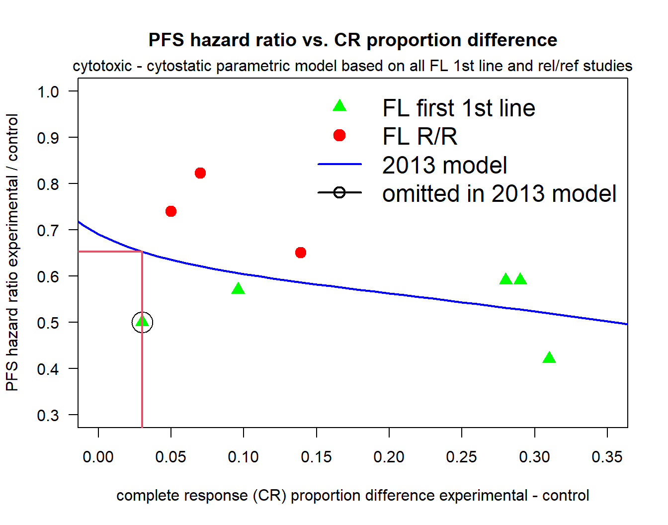

# we assume this information corresponds to 12 PFS events that were observed at the interim
nGallium <- 12 
SEGallium <- sqrt(4 / nGallium)

So based on this meta-regression model we predict that a CR proportion difference (experimental - control) of 3% corresponds to a hazard ratio for PFS of 0.652. Consequently, we quantify the knowledge of not stopping at the interim analysis based on CR in Gallium as \(X_\mathrm{Gallium} \sim N(\log 0.652, 4 / 12).\)

Goya does not stop at futility interim

We can go through the same exercise for Goya as for Gallium, see here for the details. The results are:

HRGoya <- 0.544
nGoya <- 37
SEGoya <- sqrt(4 / nGoya)

so that we quantify the knowledge of not stopping Goya at the interim based on CR as \(X_\mathrm{Goya} \sim N(\log 0.544, 4 / 37).\)

Pool all the data

So the four data sources provide four Normal densities that look as follows:

xs <- seq(-10, 10, by = 0.01)
  
## lines to plot
dCLL11   <- dnorm(xs, mean = log(HRCLL11), sd = SECLL11)
dGauss   <- dnorm(xs, mean = log(HRGauss), sd = SEGauss)
dGallium <- dnorm(xs, mean = log(HRGallium), sd = SEGallium)
dGoya    <- dnorm(xs, mean = log(HRGoya), sd = SEGoya)

all <- cbind(dCLL11, dGauss, dGallium, dGoya)
nams <- c("CLL11", "Gauss", "Gallium", "Goya")
pchs <- 17:20

## compute xlim
tmp <- apply(all, 1, max)
xli <- range(xs[tmp >= 10^-2], na.rm = TRUE)
  
par(las = 1, mar = c(4.5, 4, 3, 1))
plot(0, 0, type = "n", xlim = xli, ylim = range(all, na.rm = TRUE), xlab = "log(HR)", 
     ylab = "density", main = "Normal densities of log(HR)'s")
abline(h = 0, lty = 3)

for (i in 1:ncol(all)){
  lines(xs, all[, i], col = i + 1, lty = 1, lwd = 2)
  #points(xs, all[, i], col = grey(0.75), pch = pchs[i])
}
legend("topright", nams, lty = 1, col = 2:10, bty = "n", lwd = 2)

segments(0, 0, 0, 2, col = grey(0.75), lty = 2)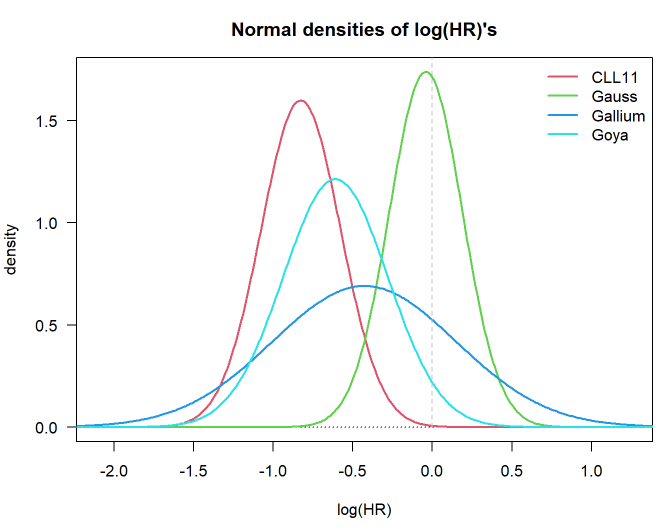

Now the question is how to synthesize this evidence? The easiest way is to simply take a weighted average of the random variables corresponding to these four densities (assuming they are independent…):

\[ X_\mathrm{data} = w_\mathrm{CLL11} X_\mathrm{CLL11} + w_\mathrm{GAUSS} X_\mathrm{GAUSS} + w_\mathrm{GALLIUM} X_\mathrm{GALLIUM}+ w_\mathrm{GOYA} X_\mathrm{GOYA}. \] However, that poses the challenge of how to choose the weights. Variuous approaches to weight selection were explored in the Gazyva program, see here for details. The conclusion was that the evidence provided by the above sources is quite sensitive to selection of these weights to that decision-makers decided NOT to update PTS based on all this evidence. So:

Event	Goya	Gallium
First discussion of trials	0.65	0.65
Update 1, Q1/2011	0.41	0.41
Update 2, Q1/2013	0.41	0.41

Back-engineer priors

However, in order to be ready to update PTS after the upcoming interim analyses on the primary endpoint of PFS in Goya and Gallium, the team back-engineered a Normal prior for the PFS HR in both trials such that PTS was equal to 0.41. To this end, the variability was assumed to correspond to the number of events observed in the respective futility interim on response (because that was the knowledge at the time of development of the prior), so that we only needed to find the mean of the Normal prior that gives a PTS of 0.41. This mean can be found through inversion of the BBP function, see tutorial on back-engineering a prior.

To do that we first need to specify the details of Gallium in terms of final analysis. For the sake of brevity we omit all the computations for Goya. These are similar to the ones for Gallium.

##---------------------------------------------------------
## Gallium: general, study specific, definitions
##---------------------------------------------------------
med.control <- 72
med.tmt <- 97.2
lam.control <- log(2) / med.control
lam.tmt <- log(2) / med.tmt

HRprotocol <- lam.tmt / lam.control
nevents <- c(248, 370)
information <- nevents / max(nevents)

# local significance levels
library(rpact)
design <- getDesignGroupSequential(sided = 2, alpha = 0.05, beta = 0.2,
                                   informationRates = information,
                                   typeOfDesign = "asOF")
zquantiles <- design$criticalValues
alphas <- 2 * (1 - pnorm(zquantiles))

# MDDs: since we are not using the number of events that a sample size computation would 
# give us we are not using rpact
# (see https://pages.github.roche.com/adaptR/adaptR-tutorials/rpactAnalysisExamples.html)
hrMDD <- exp(- qnorm(1 - alphas / 2) * sqrt(4 / nevents))
hrMDD

[1] 0.7278413 0.8127873

# quantities at final analysis
minDetectHR <- hrMDD[2]
TotEvents   <- nevents[2]

Having specified the necessary numbers of Gallium for the final analysis we can now back-compute the mean of the prior:

# invert BBP formula to get mean of prior on log(HR)
pts.initial <- 0.41
theta0 <- log(minDetectHR) - qnorm(pts.initial) * sqrt(4 / TotEvents + 4 / nGallium)

# so the prior mean on the HR scale is
exp(theta0)

[1] 0.9288581

Now let us confirm that indeed, for a prior \(N(0.93, 4 / 12)\) BBP equals 0.41. To this end, we can use the bpp package:

bpp_t2e(prior = "normal", successHR = minDetectHR, d = TotEvents,
                priorHR = exp(theta0), priorsigma = sqrt(4 / nGallium))

[1] 0.41

Event 3, Q1/2014: futility interims

The next milestone were futility interim analyses in both, Gallium and Goya. The iDMC was advised to recommend continuation of the trials if the hazard ratio was \(\le 1\). So the next task is to update the above PTS with the knowledge that HR \(\le 1\). The math for this has been derived in Rufibach et al. (2016) and is described in detail in the Tutorial Update assurance of a clinical trial after not stopping at an interim analysis.

# ---------------------------------------------------
# specifications for the interim analysis
# ---------------------------------------------------

# efficacy boundary --> no stopping for efficacy possible at this interim
effi <- 0

# futility boundary: HR = 1
futi <- 1

# futility interim happened after 111 events
nevents <- c(111, nevents)

# grid to compute densities on
thetas <- seq(0.3, 2.7, by = 0.01)

Now we can compute the updated BBP assuming the above Normal prior:

bpp1 <- bpp_1interim_t2e(prior = "normal", successHR = minDetectHR, d = nevents[c(1, 3)],
                          IntEffBoundary = effi, IntFutBoundary = futi, IntFixHR = 1, 
                          priorHR = exp(theta0), propA = 0.5, thetas = thetas, 
                          priorsigma = sqrt(4 / nGallium))
bpp1 <- bpp1$"BPP after not stopping at interim interval"
bpp1

[1] 0.7393927

This BBP of 0.74 assumes that there is no additional interim analysis planned until the final analysis. Another question of interest is What is the BBP to stop at the upcoming efficacy interim? To compute that BBP value we assume the upcoming efficacy interim is the final analysis and assume that the MDD at the efficacy interim is the hazard ratio we need to beat:

# after not stopping @ PFS futility, PTS @ efficacy interim analysis
bpp2 <- bpp_1interim_t2e(prior = "normal", successHR = hrMDD[1], d = nevents[c(1, 2)],
                          IntEffBoundary = effi, IntFutBoundary = futi, IntFixHR = 1, 
                          priorHR = exp(theta0), propA = 0.5, thetas = thetas, 
                          priorsigma = sqrt(4 / nGallium))
bpp2 <- bpp2$"BPP after not stopping at interim interval"
bpp2

[1] 0.6193727

Finally, we may be interested in What is the BBP to be significant at the final analysis, assume we will not stop at the upcoming efficacy interim? The bpp package offers a function that can take into account two interims, both for futility and/or efficacy. Note that for two interims only the generic bpp function, no wrapper functions, are available.

# first we need to define vectors of futility and efficacy interim boundaries
effi <- log(c(0, hrMDD[1]))
futi <- log(c(1, Inf))

bpp3 <- bpp_2interim(prior = "normal", interimSE = sqrt(4 / nevents[1:2]), 
                     finalSE = sqrt(4 / nevents[3]), 
                     successmean = log(hrMDD[2]), IntEffBoundary = effi, 
                     IntFutBoundary = futi, priormean = theta0, thetas = log(thetas), 
                     priorsigma = sqrt(4 / nGallium))
bpp3 <- bpp3$"BPP after not stopping at interim interval"
bpp3

[1] 0.3219431

So wrapping things up for Gallium, after this milestone we have:

Event	Details	Gallium
First discussion of trials		0.65
Update 1, Q1/2011		0.41
Update 2, Q1/2013		0.41
Update 3, Q1/2014, efficacy interims	PTS @ efficacy interim	0.62
	PoS @ final, assume no PFS efficacy	0.74
	PoS @ final, assume we pass PFS efficacy	0.32

Outcome of the program

With a hazard ratio of 0.66, Gallium stopped at the pre-specified interim analysis for efficacy.

Goya did not stop at the efficacy interim and was finally negative, with a hazard ratio of 0.92.

Final comments

This is an example for PoS update throughout the lifecycle of a drug development program. Updates were done

using external (other trials) and internal (passing of interim analyses) data,
formally within the mathematical DDCP framework and informally via PTS adjustments.

Some caveats should be mentioned:

Gauss entered with two snapshots.
Only point estimates were used, there was no formal adjustment for variability.
The estimation uncertainty in the response model was not accounted for.
iDMCs issued their recommendation taking into account the “totality of information”. Strictly speaking, we did not know whether the hazard ratios at the futility interim were strictly below 1.
The prior was “back-engineered”, not formally elicited.

All in all this was a nice exercise in applied statistics. It led to:

Directly to two methodological publications: Rufibach et al. (2016), Rufibach et al. (2016).
The R package bpp (2021).
Indirectly to two more publications: Kunzmann et al. (2021) and Kunzmann et al. (2020).

References

Kunzmann, Kevin, Michael J. Grayling, Kim May Lee, David S. Robertson, Kaspar Rufibach, and James M. S. Wason. 2021. “A Review of Bayesian Perspectives on Sample Size Derivation for Confirmatory Trials.” The American Statistician 75 (4): 424–32. https://doi.org/10.1080/00031305.2021.1901782.

Kunzmann, Kevin, Michael J. Grayling, Kim M. Lee, David S. Robertson, Kaspar Rufibach, and James M. S. Wason. 2020. “Conditional Power and Friends: The Why and How of (Un)planned, Unblinded Sample Size Recalculations in Confirmatory Trials.” https://arxiv.org/abs/2010.06567.

Rufibach, K., H. U. Burger, and M. Abt. 2016. “Bayesian Predictive Power: Choice of Prior and Some Recommendations for Its Use as Probability of Success in Drug Development.” Pharm. Stat. 15: 438–46.

Rufibach, K., P. Jordan, and M. Abt. 2016. “Sequentially updating the likelihood of success of a Phase 3 pivotal time-to-event trial based on interim analyses or external information.” J Biopharm Stat 26 (2): 191–201. http://dx.doi.org/10.1080/10543406.2014.972508.

———. 2021. Bpp: Computations Around Bayesian Predictive Power.