pi_ext1 <- 0.63
pi_ext2 <- 0.41
mean1 <- (pi_ext1 - pi_ext2)
se_ext <- sqrt(pi_ext1 * (1 - pi_ext1) / 22 + pi_ext2 * (1 - pi_ext2) / 23)Update assurance of a clinical trial after not stopping at an interim analysis: binary endpoint
Setup
We assume that DDCP at the design stage of Phase 3 trial has already been computed, as described in the corresponding tutorial. We continue analyzing the first of the two examples in the design tutorial, i.e. the one relying on the Normal approximation.
The question we are answering here is now how the two DDCP values (one for each prior), 0.74 and 0.64, change during the trial when one of the following events happens:
- External information on the treatment effect becomes available.
- An interim analysis for futility and/or efficacy for the trial of interest itself is performed, and the trial is not stopped at that interim analysis. The question then is how the knowledge of not stopping at the interim analysis changes the Bayesian predictive probability. Computations are possible for both scenarios, when the interim effect estimate is known or unknown to the sponsor.
External information becomes available
Assume an early phase trial with 22 + 23 = 45 patients on a related molecule has read out. How should we update DDCP? The trial showed the following results (in line with rpact notation index 1 always refers to intervention and 2 to control):
As discussed in Section 2.4 of Rufibach et al. (2016) the proposal is to simply update our prior distribution \(q\) with this data. If we have more than one external trial result we can either do this updating sequentially or by first meta-analyzing the multiple trials.
# ----------------------------------
# Normal prior:
# ----------------------------------
up1 <- NormalNormalPosterior(datamean = mean1, sigma = se_ext, n = 1, nu = priormean,
                             tau = sd0)
bpp1 <- bpp_binary(prior = "normal", successdelta = mdd, pi1 = pi1, n1 = n1,
                   pi2 = pi2, n2 = n2, priormean = up1$postmean, priorsigma = up1$postsigma)

# Normal prior
up1
$postmean
[1] 0.2094921
$postsigma
[1] 0.1001014bpp1[1] 0.8203384We find that updating the prior with the information from the external trial changes our Normal prior with mean = 0.20 and standard deviation 0.14 to a posterior with mean = 0.21 and increases DDCP from the initial 0.74 to 0.82.
# ----------------------------------
# pessimistic prior
# ----------------------------------
finalSE <- sqrt(pi2 * (1 - pi2) / n2 + pi1 * (1 - pi1) / n1)
bpp1_1 <- 1 - integrate(FlatNormalPosterior, lower = Inf, upper = Inf, successmean = mdd,
                        finalSE = finalSE, interimmean = mean1, interimSE = se_ext,
                        priormean = priormeanflat, width = width1, height = height1)$value

# flat prior
bpp1_1
[1] 0.7732243We find that updating the prior with the information from the external trial increases DDCP from the initial 0.64 to 0.23 if we use the pessimistic prior.
Update the prior distribution after not stopping at an interim analysis
Now, the next milestone in our trial of interest is an interim analysis for both, futility and efficacy:
# ---------------------------------------------------
# specifications for the interim analysis
# ---------------------------------------------------

# local significance levels based on rpact output
alphas <- 2 * design$stageLevels
alphas
[1] 0.003050646 0.048999543# number of patients
n1_int <- ceiling(as.vector(sampleSize$numberOfSubjects1)[1])
n2_int <- ceiling(as.vector(sampleSize$numberOfSubjects2)[1])
c(n1_int, n2_int)[1] 87 87# MDDs at interim and final based on rpact output
mdd <- as.vector(sampleSize$criticalValuesEffectScaleUpper)
mdd[1] 0.2232384 0.1056952# efficacy boundary --> mdd at interim
effi <- mdd[1]
# futility boundary --> chosen informally
futi <- 0The interim analysis is planned after 174 patients (both arms combined), using local significance levels of \(\alpha_{inte} \ = \ 0.003\) for the interim and \(\alpha_{fin} \ = \ 0.049\) for the final analysis. From these local significance levels, together with the number of patients at each analysis, the minimal detectable differences (the proportion differences corresponding to the critical values of the hypothesis test, MDD) can be derived. These are 0.22 and 0.11.
In addition to the interim efficacy analysis, assume that a futility analysis was pre-specified in the iDMC charter, with interim futility boundary of \(\theta_{fut} \ = \ 0\). Thus, if the trial is not stopped at the interim analysis, we may assume for the mean difference estimate at the interim analysis that \({\hat \theta}_{inte} \in [\theta_{fut}, \theta_{eff}] \ = \ [0, 0.22]\).
Now we are interested how DDCP changes if we do not stop at that interim analysis. For illustrative purposes, we assess various scenarios: the interim is set up with futility and efficacy boundary, only one of the two, and we also provide updates using conditional power for the two extreme cases, namely that the estimate at the interim was known to be either equal to the futility or the efficacy boundary. Let us start with the Normal prior. We use the protocol assumed proportions to estimate a standard error.
# ----------------------------------
# compute bpp after not stopping at interim, for Normal prior and various
# assumptions on the amount of information we learn at the interim
#
# Note that if we are only interested on a "blinded" or "interval" update we can set
# IntFix to an arbitrary value. Below, this is the case whenever we set IntFix = 1
# ----------------------------------

# assuming we do not stop at a blinded interim analysis for futility and efficacy:
bpp3.tmp <- bpp_1interim_binary(prior = "normal", successdelta = mdd[2], pi1 = pi1,
                                n1 = c(n1_int, n1), pi2 = pi2, n2 = c(n2_int, n2),
                                IntEffBoundary = effi, IntFutBoundary = futi, IntFix = 1,
                                priormean = up1$postmean, propA = 0.5, thetas = thetas,
                                priorsigma = up1$postsigma)
bpp3 <- bpp3.tmp$"BPP after not stopping at interim interval"
post3 <- bpp3.tmp$"posterior density interval"

# assuming we do not stop at a blinded interim analysis for efficacy only:
bpp3_effi_only <- bpp_1interim_binary(prior = "normal", successdelta = mdd[2], pi1 = pi1,
                                n1 = c(n1_int, n1), pi2 = pi2, n2 = c(n2_int, n2),
                                IntEffBoundary = effi, IntFutBoundary = -Inf, IntFix = 1,
                                priormean = up1$postmean, propA = 0.5, thetas = thetas,
                                priorsigma = up1$postsigma)$"BPP after not stopping at interim interval"

# assuming we do not stop at a blinded interim analysis for futility only:
bpp3_futi_only <- bpp_1interim_binary(prior = "normal", successdelta = mdd[2], pi1 = pi1,
                                n1 = c(n1_int, n1), pi2 = pi2, n2 = c(n2_int, n2),
                                IntEffBoundary = Inf, IntFutBoundary = futi, IntFix = 1,
                                priormean = up1$postmean, propA = 0.5, thetas = thetas,
                                priorsigma = up1$postsigma)$"BPP after not stopping at interim interval"

# assuming we do not stop at an unblinded interim where we observe exactly the efficacy boundary
# (IntFix = effi):
bpp4.tmp <- bpp_1interim_binary(prior = "normal", successdelta = mdd[2], pi1 = pi1,
                                n1 = c(n1_int, n1), pi2 = pi2, n2 = c(n2_int, n2),
                                IntEffBoundary = Inf, IntFutBoundary = -Inf, IntFix = effi,
                                priormean = up1$postmean, propA = 0.5, thetas = thetas,
                                priorsigma = up1$postsigma)
bpp4 <- bpp4.tmp$"BPP after not stopping at interim exact"[2, 1]
post4 <- bpp4.tmp$"posterior density exact"[, 1]

# assuming we do not stop at an unblinded interim where we observe exactly the futility boundary
# (IntFix = futi):
bpp5.tmp <- bpp_1interim_binary(prior = "normal", successdelta = mdd[2], pi1 = pi1,
                                n1 = c(n1_int, n1), pi2 = pi2, n2 = c(n2_int, n2),
                                IntEffBoundary = Inf, IntFutBoundary = -Inf, IntFix = futi,
                                priormean = up1$postmean, propA = 0.5, thetas = thetas,
                                priorsigma = up1$postsigma)
bpp5 <- bpp5.tmp$"BPP after not stopping at interim exact"[2, 1]
post5 <- bpp5.tmp$"posterior density exact"     # same as post4[, 2]
And the same for the pessimistic prior:
# ----------------------------------
# compute bpp after not stopping at interim, for pessimistic prior and various
# assumptions on the amount of information we learn at the interim
# here we do not assume an update with external studies, i.e. we use the
# initial prior
# ----------------------------------

# assuming we do not stop at a blinded interim analysis for futility and efficacy:
bpp3.tmp_1 <- bpp_1interim_binary(prior = "flat", successdelta = mdd[2], pi1 = pi1,
                                  n1 = c(n1_int, n1), pi2 = pi2, n2 = c(n2_int, n2),
                                  IntEffBoundary = effi, IntFutBoundary = futi, IntFix = 1,
                                  priormean = priormean, propA = 0.5, thetas = thetas,
                                  width = width1, height = height1)

bpp3_1 <- bpp3.tmp_1$"BPP after not stopping at interim interval"
post3_1 <- bpp3.tmp_1$"posterior density interval"

# assuming we do not stop at a blinded interim analysis for efficacy only:
bpp3_1_effi_only <- bpp_1interim_binary(prior = "flat", successdelta = mdd[2], pi1 = pi1,
                                        n1 = c(n1_int, n1), pi2 = pi2, n2 = c(n2_int, n2),
                                        IntEffBoundary = effi, IntFutBoundary = -Inf, IntFix = 1,
                                        priormean = priormean, propA = 0.5, thetas = thetas,
                                        width = width1, height =
                                          height1)$"BPP after not stopping at interim interval"

# assuming we do not stop at a blinded interim analysis for futility only:
bpp3_1_futi_only <- bpp_1interim_binary(prior = "flat", successdelta = mdd[2], pi1 = pi1,
                                        n1 = c(n1_int, n1), pi2 = pi2, n2 = c(n2_int, n2),
                                        IntEffBoundary = Inf, IntFutBoundary = futi, IntFix = 1,
                                        priormean = priormean, propA = 0.5, thetas = thetas,
                                        width = width1, height =
                                          height1)$"BPP after not stopping at interim interval"

# assuming we do not stop at an unblinded interim where we observe exactly the efficacy boundary
# (IntFix = effi):
bpp4_1.tmp <- bpp_1interim_binary(prior = "flat", successdelta = mdd[2], pi1 = pi1,
                                        n1 = c(n1_int, n1), pi2 = pi2, n2 = c(n2_int, n2),
                                        IntEffBoundary = Inf, IntFutBoundary = -Inf, IntFix = effi,
                                        priormean = priormean, propA = 0.5, thetas = thetas,
                                        width = width1, height = height1)
bpp4_1 <- bpp4_1.tmp$"BPP after not stopping at interim exact"[2, 1]
post4_1 <- bpp4_1.tmp$"posterior density exact"

# assuming we do not stop at an unblinded interim where we observe exactly the efficacy boundary
# (IntFix = futi):
bpp5_1.tmp <- bpp_1interim_binary(prior = "flat", successdelta = mdd[2], pi1 = pi1,
                                        n1 = c(n1_int, n1), pi2 = pi2, n2 = c(n2_int, n2),
                                        IntEffBoundary = Inf, IntFutBoundary = -Inf, IntFix = futi,
                                        priormean = priormean, propA = 0.5, thetas = thetas,
                                        width = width1, height = height1)
bpp5_1 <- bpp5_1.tmp$"BPP after not stopping at interim exact"[2, 1]
post5_1 <- bpp5_1.tmp$"posterior density exact"
Posterior densities
The resulting posteriors after the update with the external trial is depicted below. We also add to the figures the posterior after not stopping at the interim analysis that considers the efficacy and futility boundary, i.e. we may assume that \[{\hat \theta}_{inte} \in [\theta_{fut}, \theta_{eff}] \ = \ [0, 0.22].\]
These figures adapt Figure 1 in Rufibach et al. (2016) to our setup.
par(las = 1, mar = c(4.5, 4.5, 4.5, 1), mfrow = c(1, 2), cex = 0.8)
leg <- c("prior", "posterior after external trial",
         "posterior after external trial and\nnot stopping at interim")

# ----------------------------------
# Normal prior:
# ----------------------------------
xli <- priormean + 0.5 * c(-1, 1)
yli <- c(0, 8)
plot(0, 0, type = "n", xlim = xli, ylim = yli, xlab = "proportion difference", ylab = "density",
     main = "Normal prior density for\nproportion difference")
abline(h = 0, lty = 3)
lines(thetas, dnorm(thetas, mean = priormean, sd = sd0), col = 2, lwd = 2)
lines(thetas, dnorm(thetas, mean = up1$postmean, sd = up1$postsigma), col = 3, lwd = 2)
lines(thetas, post3, col = 1, lwd = 2)
legend("topleft", leg, lty = 1, col = c(2:3, 1), bty = "n", lwd = 2)

# ----------------------------------
# pessimistic prior:
# ----------------------------------

# first we have to compute the posteriors after the external updates:
flatpost1 <- rep(NA, length(thetas))
for (i in 1:length(thetas)){
  flatpost1[i] <- estimate_posterior(x = thetas[i], prior = "flat", interimmean = mean1,
                                     interimSE = se_ext, priormean = priormeanflat, width = width1,
                                     height = height1)
}

plot(0, 0, type = "n", xlim = xli, ylim = yli, xlab = "proportion difference", ylab = "density",
     main = "Pessimistic prior density for\nproportion difference")
abline(h = 0, lty = 3)
lines(thetas, dUniformNormalTails(thetas, mu = priormeanflat, width = width1, height = height1),
      lwd = 2, col = 2)
lines(thetas, flatpost1, col = 3, lwd = 2)
lines(thetas, post3_1, col = 1, lwd = 2)

legend("topleft", leg, lty = 1, col = c(2:3, 1), bty = "n", lwd = 2)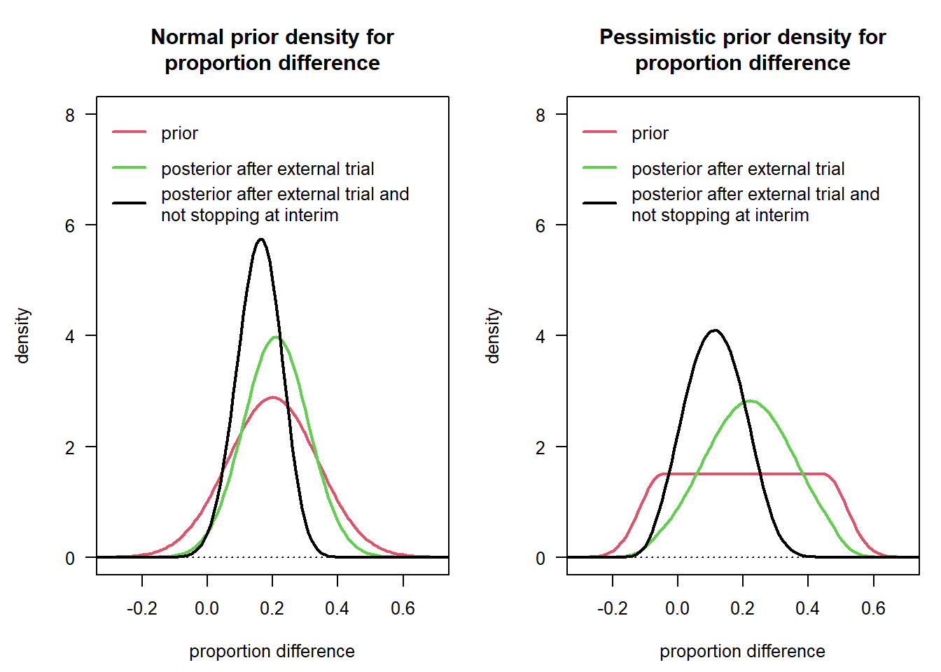
Next, we also provide the posteriors after updating with the interim information assuming the effect estimate at the interim came to lie on one of the interim boundaries:
par(las = 1, mar = c(4.5, 4.5, 4.5, 1), mfrow = c(1, 2), cex = 0.8)

# ----------------------------------
# Normal prior:
# ----------------------------------
plot(0, 0, type = "n", xlim = xli, ylim = yli, xlab = "proportion difference", ylab = "density",
     main = "Normal prior density for\nproportion difference")
abline(h = 0, lty = 3)
lines(thetas, post3, col = 1, lwd = 2)
lines(thetas, post4, col = 2, lwd = 2)
lines(thetas, post5, col = 3, lwd = 2)
leg2 <- c("interval knowledge", expression(hat(theta)*" = efficacy boundary"),
          expression(hat(theta)*" = futility boundary"))
legend("topleft", leg2, lty = 1, col = 1:3, lwd = 2, bty = "n",
       title = "posterior after not stopping at interim,")

# ----------------------------------
# pessimistic prior:
# ----------------------------------
plot(0, 0, type = "n", xlim = xli, ylim = yli, xlab = "proportion difference", ylab = "density",
     main = "Pessimistic prior density for\nproportion difference")
abline(h = 0, lty = 3)
lines(thetas, post3_1, col = 1, lwd = 2)
lines(thetas, post4_1, col = 2, lwd = 2)
lines(thetas, post5_1, col = 3, lwd = 2)
legend("topleft", leg2, lty = 1, col = 1:3, lwd = 2, bty = "n",
       title = "posterior after not stopping at interim,")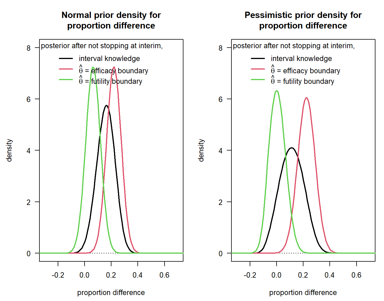
Table 1 in Rufibach et al. (2016)
Finally, we collect all the results computed above in one table, adapting Table 1 in Rufibach et al. (2016).
mat <- matrix(NA, ncol = 2, nrow = 9)
mat[, 1] <- c(pnorm2, pnorm1, bpp0, bpp1, bpp3, bpp3_futi_only, bpp3_effi_only, bpp4, bpp5)
mat[, 2] <- c(flat2, flat1, bpp0_1, bpp1_1, bpp3_1, bpp3_1_futi_only, bpp3_1_effi_only,
              bpp4_1, bpp5_1)
colnames(mat) <- c("Normal prior", "Flat prior")
rownames(mat) <- c(paste("Probability for proportion difference to be $\\le$ ", lims[1], sep = ""),
  paste("Probability for proportion difference to be $\\ge$ ", lims[2], sep = ""),
"DDCP based on prior distribution", "DDCP after external trial",
"DDCP after external trial and not stopping at interim, assuming $\\hat \\theta \\in [\\theta_{fut}, \\theta_{eff}]$",
"DDCP after external trial and not stopping at interim, assuming $\\hat \\theta \\in [\\theta_{fut}, \\infty, ]$",
"DDCP after external trial and not stopping at interim, assuming $\\hat \\theta \\in [-\\infty, \\theta_{eff}]$",
"DDCP after external trial and not stopping at interim, assuming $\\hat \\theta = \\theta_{eff}$",
"DDCP after external trial and not stopping at interim, assuming $\\hat \\theta = \\theta_{fut}$")
mat <- as.data.frame(apply(mat, 1:2, disp, 4))
knitr::kable(mat)| Normal prior | Flat prior | |
|---|---|---|
| Probability for proportion difference to be \(\le\) 0 | 0.6413 | 0.5750 |
| Probability for proportion difference to be \(\ge\) 0.15 | 0.0738 | 0.2000 |
| DDCP based on prior distribution | 0.7381 | 0.6415 |
| DDCP after external trial | 0.8203 | 0.7732 |
| DDCP after external trial and not stopping at interim, assuming \(\hat \theta \in [\theta_{fut}, \theta_{eff}]\) | 0.7239 | 0.5294 |
| DDCP after external trial and not stopping at interim, assuming \(\hat \theta \in [\theta_{fut}, \infty, ]\) | 0.8545 | 0.8036 |
| DDCP after external trial and not stopping at interim, assuming \(\hat \theta \in [-\infty, \theta_{eff}]\) | 0.6708 | 0.3297 |
| DDCP after external trial and not stopping at interim, assuming \(\hat \theta = \theta_{eff}\) | 0.9992 | 0.9987 |
| DDCP after external trial and not stopping at interim, assuming \(\hat \theta = \theta_{fut}\) | 0.0118 | 0.0035 |
Update of DDCP when not stopping the trial in two blinded interim analyses
The theory developed in Rufibach et al. (2016) can straightforwardly be extended to accomodate more than one interim analysis. This is illustrated in the tutorial for interim updates for a T2E endpoint.
Exact computations using the binomial distribution
As discussed in the design tutorial for a binary endpoint the Normal approximation used above might not work terribly well in some instances. So what to do if we are in this situation and want to update DDCP after an interim? Currently, there is no implementation of the exact computation available for external or internal updates. The recommendation is that if you are in an extreme case where design DDCP based on Normal approximation and exact binomial computation are relevantly different (as in the second example in the design tutorial for a binary endpoint) then adjust DDCP in line with what happens to DDCP using the Normal approximation. This is a pragmatic fix in absence of a proper “exact” implementation. Alternatively, if you really want the exact results also for the update you can run simulations.
References
Rufibach, K., P. Jordan, and M. Abt. 2016. “Sequentially updating the likelihood of success of a Phase 3 pivotal time-to-event trial based on interim analyses or external information.” J Biopharm Stat 26 (2): 191–201. http://dx.doi.org/10.1080/10543406.2014.972508.