# Load bpp
library(bpp)

# load rpact
library(rpact)Compute assurance at the design stage of a clinical trial: binary endpoint
Purpose
This document provides code to compute assurance at the design stage of a clinical trial for a binary primary endpoint. We have designing a Phase 3 trial in mind, but the concepts are equally well applicable when designing a Phase 2 trial. In the latter case, the success criterion might be somewhat different.
Setup
Load packages:
Our trial of interest
We assume that we plan a 1:1 randomized trial for a binary endpoint, so the effect measure we are interested in is the difference \(\delta = \pi_1 - \pi_2\) in proportions between two arms, with (in accordance with rpact notation) \(\pi_1\) is the proportion in the intervention and \(\pi_2\) in the control arm. We further assume that a higher proportion is better, like e.g. response in oncology. The trial will have one interim analysis after 50% of information. We start with defining the parameters of this pivotal trial. Note that the success probability part in the generic function bpp is parametrized such that we always look at the probability \(P(\hat \delta_\text{fin} \le \delta_\text{suc})\), see general methodology. However, the bpp package contains a wrapper function bpp_binary for the scenario with “higher proportion is better” which we use here.
# ---------------------------------------------------
# specifications of the pivotal trial
# ---------------------------------------------------

# set up a group-sequential design with an interim after 50% of information
# significance levels at final analysis
design <- getDesignGroupSequential(sided = 2, alpha = 0.05, beta = 0.2,
                                   informationRates = c(0.5 ,1),
                                   typeOfDesign = "asOF")

# number of patients needed per arm
pi2 <- 0.45             # proportion in control arm
delta <- 0.15           # targeted difference to have 80% power
pi1 <- pi2 + delta      # proportion in intervention arm
sampleSize <- getSampleSizeRates(pi2 = pi2, pi1 = pi1, design)
n1 <- ceiling(sampleSize$numberOfSubjects1[2, 1])
n2 <- ceiling(sampleSize$numberOfSubjects2[2, 1])
c(n1, n2)
[1] 174 174# MDD at final
mdd <- sampleSize$criticalValuesEffectScaleUpper[2, 1]
mdd[1] 0.1056952Define the prior distribution
As a next step we define the parameters of the prior density \(q(\theta)\). For a discussion of aspects of prior choice also see the tutorial on choice of prior.
Normal prior
# ----------------------------------
# mean and sd of Normal prior:
# ----------------------------------
pi20 <- 0.44
pi10 <- 0.64
priormean <- (pi10 - pi20)
priormean
[1] 0.2# standard error of that proportion difference
n0 <- 50
sd0 <- sqrt(pi20 * (1 - pi20) / (n0 / 2) + pi10 * (1 - pi10) / (n0 / 2))The above prior could e.g. result from a Phase 2 trial with observed proportion difference of 0.2 (which we chose not to attenuate) based on observed proportions of 0.44 and 0.64 in a 1:1 randomized Phase II trial with 50 patients. The resulting density function is depicted as red line in the figure below.
To better understand the properties of this prior we can compute a few probabilities of interest:
lims <- c(0, delta)
pnorm1 <- pnorm(lims[1], mean = priormean, sd = sd0)
pnorm2 <- 1 - pnorm(lims[2], mean = priormean, sd = sd0)
c(pnorm1, pnorm2)
[1] 0.07377901 0.64134370So the probability for the proportion difference to be below 0 or above 0.15 amounts to 0.07 and 0.64, respectively. The prior thus allows for a 7% probability that the treatment effect may be on the harmful side.
# ----------------------------------
# parameters of pessimistic, or flat, prior:
# ----------------------------------
priormeanflat <- priormean
width1 <- 0.5
height1 <- 1.5
The above code specifies a more pessimistic alternative prior, see this tutorial for details on how to specify such a prior. This may potentially more accurately reflect the (absence of) knowledge about the treatment effect at the design stage or could be used as a kind of sensitivity analysis. Such a prior has e.g. been used when quantifying the success probability at the design stage in the MIRROS case study, for a time-to-event endpoint though.
To specify a pessimistic prior we retain the lower tail of the Normal prior above but move the upper tail slightly to the right, allowing for a plateau in the center of the distribution. To compute the probabilities to be below 0 or above 0.15 we have to integrate over the density function of the pessimistic prior. The function for this density is available in the package bpp.
flat1 <- integrate(dUniformNormalTails, lower = -Inf, upper = lims[1],
                   mu = priormeanflat, width = width1, height = height1)$value
flat2 <- integrate(dUniformNormalTails, lower = lims[2], upper = Inf,
                   mu = priormeanflat, width = width1, height = height1)$value
c(flat1, flat2)
[1] 0.1999999 0.5750003This leads to a 20% probability for the true proportion difference to be below 0. The red line in the figure below illustrates this alternative prior.
par(las = 1, mar = c(4.5, 4.5, 2, 1), mfrow = c(1, 1))
xli <- priormean + 0.5 * c(-1, 1)
yli <- c(0, 3.2)
plot(0, 0, type = "n", xlim = xli, ylim = yli, xlab = "proportion difference", ylab = "density",
     main = "Normal and pessimistic prior density for proportion difference")
abline(h = 0, lty = 3)

# grid to compute densities on
thetas <- seq(-1, 1, by = 0.01)

lines(thetas, dnorm(thetas, mean = priormean, sd = sd0), col = 2, lwd = 2)
lines(thetas, dUniformNormalTails(thetas, mu = priormeanflat,
                                  width = width1, height = height1), lwd = 2, col = 3)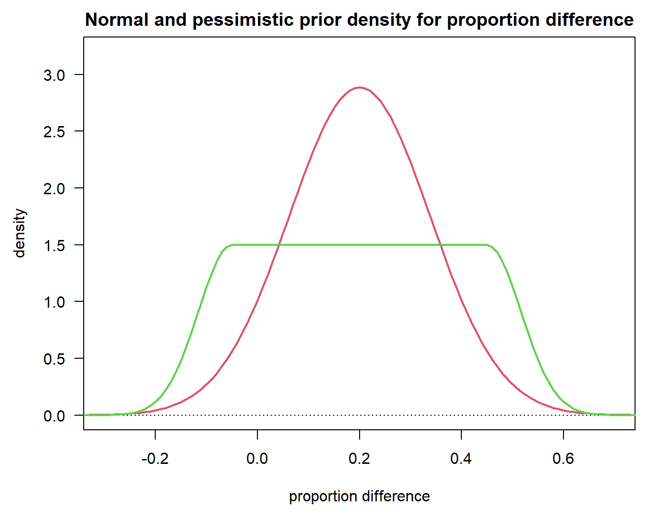
DDCP at the beginning of the trial
Having specified one or more priors together with the details of the trial of interest we can now quite easily compute the corresponding DDCP values.
# ----------------------------------
# Normal prior:
# ----------------------------------
bpp0 <- bpp_binary(prior = "normal", successdelta = mdd, pi1 = pi1, n1 = n1,
                   pi2 = pi2, n2 = n2, priormean = priormean, priorsigma = sd0)

# ----------------------------------
# pessimistic prior:
# ----------------------------------
bpp0_1 <- bpp_binary(prior = "flat", successdelta = mdd, pi1 = pi1, n1 = n1,
                     pi2 = pi2, n2 = n2, priormean = priormeanflat,
                     width = width1, height = height1)

c(bpp0, bpp0_1)
[1] 0.7381444 0.6414558Note that the arguments for bpp differ, depending on which prior you want to compute DDCP for. We find that based on our priors and the specifications for the trial of interest we get values of 0.74 and 0.64. These are our BBP values at the design stage of the trial.
Exact computations using the binomial distribution
The Normal approximation used above might not work terribly well for either
small sample sizes of the Phase 3 and/or
when \(\pi_1, \pi_2\) are close to zero or one. The usual rule-of-thumb is that the Normal approximation is accurate enough if the expected number of responders and non-responders in each arm is \(\ge 5\), i.e.
- \(n_1 \cdot \pi_1\),
- \(n_1 \cdot (1 - \pi_1)\),
- \(n_2 \cdot \pi_2\),
- and \(n_2 \cdot (1 - \pi_2)\)
are all \(\geq 5\).
If that is not fulfilled exact results can be obtained by replacing the above integral through a sum over binomial probabilities. This generalizes the methods used for phase 1b trials in Unicycle to two samples, albeit with a different success criterion. The details of the computations below are given e.g. in Kundu et al. (2021).
Before Phase 2 we assume that \(\pi_i \sim \beta(a_i, b_i), i = 1, 2\) follow \(\beta\) prior distributions. In Phase 2 we then observe \(r_{21}\) responders among \(n_{21}\) patients in the intervention and \(r_{22}\) responders among \(n_{22}\) patients in the control arm. Using the standard beta-binomial model the priors are updated to posteriors \(\beta(a_i + r_{2i}, b_i + n_{2i} - r_{2i}), i = 1, 2\). To compute DDCP we also need an exact power part, i.e. we are interested in \(P(\hat \delta > \text{MDD})\). Recalling that \(n_1, n_2\) are the sample sizes of the Phase 3 trial in the intervention and control group and \(X_i \sim \text{Bin}(\pi_i, n_i)\) are binomial random variables counting the responders in Phase 3, this can be computed exactly as follows: \[\begin{align*} P(\hat \delta > \text{MDD}) & = 1 - P(\hat \pi_1 - \hat \pi_2 \le \text{MDD}) \\ & = 1 - \sum_{i=0}^{n_1} P(\hat \pi_1 - \hat \pi_2 \le \text{MDD} | X_1 = i)P(X_1 = i) \\ & = 1 - \sum_{i=0}^{n_1} P(X_1 / n_1 - X_2 / n_2 \le \text{MDD} | X_1 = i)P(X_1 = i) \\ & = 1 - \sum_{i=0}^{n_1} P(i / n_1 - X_2 / n_2 \le \text{MDD} )P(X_1 = i) \\ & = 1 - \sum_{i=0}^{n_1} \Bigl[1 - P(X_2 < n_2 (i / n_1 - \text{MDD}) )\Bigr]P(X_1 = i) . \end{align*}\]
In theory, one could now integrate over this power function multiplied by \(\beta\)-posterior densities of \(\pi_1\) and \(\pi_2\). For simplicity we evaluate this integral through simulation as follows:
set.seed(2021)

# number of simulations to approximate integration
M <- 10 ^ 5

# priors before Phase 2: beta(a1, b1) refers to intervention,
# beta(a2, b2) to control
# we take here uniform priors to be uninformative and match
# the approximate analysis of above
a1 <- 1
b1 <- 1
a2 <- 1
b2 <- 1
So we claim here that a \(\beta(1, 1)\) prior is uninformative, and that is true as long as the number of responses in Phase 2 is not very small. If the latter is the case the prior may play a big role and even \(\beta(1, 1)\) may become “informative” (although there is never such a thing as an “uninformative” prior!). If you are in such a situation you might want to consider choosing something like \(\alpha = \beta = 1/3\) (put forward in Kerman (2011)) or even \(\alpha = \beta = 0.001\). In any case, a symmetric prior (i.e. \(\alpha = \beta\)) is recommended and if you have very few responses in Phase 2 the prior unavoidable will have an impact on your posterior.
# response and number of patients in Phase 2
# these frequencies correspond to pi10 and pi20 above
r21 <- 16
n21 <- 25
r22 <- 11
n22 <- 25

# posterior after Phase 2 - simply beta-updating
pi21 <- rbeta(M, a1 + r21, b1 + n21 - r21)
pi22 <- rbeta(M, a2 + r22, b2 + n22 - r22)

# compute power for every simulated pair and average
ddcp_m <- rep(NA, M)
i <- 0:n1

# in the last inequality above we have a "<" sign. Subtracting a small number in the first
# argument of pbinom achieves this since pbinom rounds down the first argument
# when it is not an integer
q <- n2 * i / n1 - n2 * mdd - 1e-10
for (m in 1:M){
  ddcp_m[m] <- 1 - sum((1 - pbinom(q = q, size = n2, p = pi22[m])) *
                         dbinom(x = i, size = n1, p = pi21[m]))
}

ddcp <- mean(ddcp_m)
ddcp
[1] 0.7125349So we compute a DDCP of 0.713, which is close to the 0.738 from above that was computed using the Normal approximation. This is not a surprise, as for the exact computation we assume a non-informative prior which mimicks the Normal approximation analysis from above. So the difference between 0.713 and 0.738 is basically caused by the difference between the Normal approximation and the exact binomial computation.
Let us look at an example where we suspect that the two approaches differ: Namely, for small proportions and a small Phase 3.
set.seed(2021)

# small Phase 3 trial
pi2_2 <- 0.01               # proportion in control arm
delta_2 <- 0.2              # targeted difference to have 80% power
pi1_2 <- pi2_2 + delta_2    # proportion in intervention arm
sampleSize_2 <- getSampleSizeRates(pi2 = pi2_2, pi1 = pi1_2, design)
n1_2 <- ceiling(sampleSize_2$numberOfSubjects1[2, 1])
n2_2 <- ceiling(sampleSize_2$numberOfSubjects2[2, 1])
c(n1_2, n2_2)
[1] 38 38# MDD at final
mdd_2 <- sampleSize_2$criticalValuesEffectScaleUpper[2, 1]
mdd_2[1] 0.1138069# recompute Normal prior specifications
pi10 <- 0.26
pi20 <- 0.02
priormean_2 <- (pi10 - pi20)
sd02 <- sqrt(pi20 * (1 - pi20) / (n0 / 2) + pi10 * (1 - pi10) / (n0 / 2))
# DDCP for this trial using the same Normal prior as above
bpp1 <- bpp_binary(prior = "normal", successdelta = mdd_2, pi1 = pi1_2, n1 = n1_2,
pi2 = pi2_2, n2 = n2_2, priormean = priormean_2, priorsigma = sd02)
bpp1[1] 0.8648318# response and number of patients in Phase 2
r21 <- 5
n21 <- 25
r22 <- 0
n22 <- 25
# posterior after Phase 2 - simply beta-updating
pi21 <- rbeta(M, a1 + r21, b1 + n21 - r21)
pi22 <- rbeta(M, a2 + r22, b2 + n22 - r22)
# compute power for every simulated pair and average
ddcp_m <- rep(NA, M)
i <- 0:n1_2
q <- n2_2 * (i / n1_2 - mdd_2)
for (m in 1:M){
ddcp_m[m] <- 1 - sum((1 - pbinom(q = q, size = n2_2, p = pi22[m])) *
dbinom(x = i, size = n1_2, p = pi21[m]))
}
ddcp1 <- mean(ddcp_m)
ddcp1[1] 0.7151382So in this extreme scenario we get 0.865 using the Normal approximation and 0.715 using the exact computation, so quite a discrepancy. In such extreme scenarios it is therefore advisable to use the exact computation at the design stage.
References
Kerman, Jouni. 2011. “Neutral noninformative and informative conjugate beta and gamma prior distributions.” Electronic Journal of Statistics 5 (none): 1450–70. https://doi.org/10.1214/11-EJS648.
Kundu, Madan G., Sandipan Samanta, and Shoubhik Mondal. 2021. “An Introduction to the Determination of the Probability of a Successful Trial: Frequentist and Bayesian Approaches.” https://arxiv.org/abs/2102.13550.